Shrink Coefficient of Multiple correlation
Dongyue Xie
2019-01-15
Last updated: 2019-01-16
workflowr checks: (Click a bullet for more information)-
✔ R Markdown file: up-to-date
Great! Since the R Markdown file has been committed to the Git repository, you know the exact version of the code that produced these results.
-
✔ Environment: empty
Great job! The global environment was empty. Objects defined in the global environment can affect the analysis in your R Markdown file in unknown ways. For reproduciblity it’s best to always run the code in an empty environment.
-
✔ Seed:
set.seed(20180501)The command
set.seed(20180501)was run prior to running the code in the R Markdown file. Setting a seed ensures that any results that rely on randomness, e.g. subsampling or permutations, are reproducible. -
✔ Session information: recorded
Great job! Recording the operating system, R version, and package versions is critical for reproducibility.
-
Great! You are using Git for version control. Tracking code development and connecting the code version to the results is critical for reproducibility. The version displayed above was the version of the Git repository at the time these results were generated.✔ Repository version: 5045f0f
Note that you need to be careful to ensure that all relevant files for the analysis have been committed to Git prior to generating the results (you can usewflow_publishorwflow_git_commit). workflowr only checks the R Markdown file, but you know if there are other scripts or data files that it depends on. Below is the status of the Git repository when the results were generated:
Note that any generated files, e.g. HTML, png, CSS, etc., are not included in this status report because it is ok for generated content to have uncommitted changes.Ignored files: Ignored: .DS_Store Ignored: .Rhistory Ignored: .Rproj.user/ Ignored: data/.DS_Store Untracked files: Untracked: analysis/chipexoeg.Rmd Untracked: analysis/efsd.Rmd Untracked: analysis/talk1011.Rmd Untracked: data/chipexo_examples/ Untracked: data/chipseq_examples/ Untracked: talk.Rmd Untracked: talk.pdf Unstaged changes: Modified: analysis/binomial.Rmd Modified: analysis/fda.Rmd Modified: analysis/index.Rmd Modified: analysis/sigma.Rmd
Expand here to see past versions:
| File | Version | Author | Date | Message |
|---|---|---|---|---|
| Rmd | 5045f0f | Dongyue Xie | 2019-01-16 | wflow_publish(“analysis/r2.Rmd”) |
| html | a17b894 | Dongyue Xie | 2019-01-16 | Build site. |
| Rmd | 63ff335 | Dongyue Xie | 2019-01-16 | wflow_publish(“analysis/r2.Rmd”) |
| html | 1d90590 | Dongyue Xie | 2019-01-15 | Build site. |
| Rmd | 3f6cd72 | Dongyue Xie | 2019-01-15 | wflow_publish(“analysis/r2.Rmd”) |
| html | 265a2bb | Dongyue Xie | 2019-01-15 | Build site. |
| Rmd | 15730f5 | Dongyue Xie | 2019-01-15 | wflow_publish(“analysis/r2.Rmd”) |
Background
In multiple linear regression \(y=X\beta+\epsilon\), where \(y\in R^n\), \(X\in R^{n\times p}\) whose first column is a 1 vector, and \(\epsilon\sim N(0,\sigma^2I_n)\).
Definition of ANOVA terms:
- Total sum of squares \(SST=y^Ty-\frac{1}{n}Y^T11^Ty\) where \(1\) is \(n\times 1\) 1 vector. df=n-1
- Error sum of squares \(SSE=y^T(I-H)y\) where \(H\) is hat matrix defined as \(X(X^TX)^{-1}X^T\). df=n-p
Regression sum of squares \(SSR=\Sigma_i(\hat y_i-\bar y)^2=y^T(H-\frac{1}{n}11^T)y\). df=p-1
\(MSE=\frac{SSE}{n-p}\), \(E(MSE)=\sigma^2\); \(MSR=\frac{SSR}{p-1}\), \(E(MSR)=\sigma^2+nonnegative.quantity\)
\(\frac{MSR}{MSE}\sim F_{df_1=p-1,df_2=n-p}\).
Definition of Coefficient of Multiple correlation \(R^2\):
The proportion of the total sum of squares due to regression is \(R^2=\frac{SSR}{SST}=1-\frac{SSE}{SST}\); Adjusted R squared proposed by Ezekiel (1930): \(R_a^2=1-\frac{n-1}{n-p}\frac{SSE}{SST}\), mainly to correct 1. Adding a variable x to the model increases \(R^2\); 2. When all \(\beta\)s except intercept are 0, \(E(R^2)=\frac{p-1}{n-1}\)
Shrink \(R^2\)
Rewrite adjusted \(R^2\) as \(R_a^2=1-\frac{n-1}{n-p}\frac{SSE}{SST}=1-\frac{SSE/(n-p)}{SST/(n-1)}=1-\frac{\hat\sigma_\epsilon^2}{\hat\sigma^2_y}\) where \(\hat\sigma_\epsilon^2\) is the estimate of \(\sigma^2\) and \(\hat\sigma^2_y\) is the estimated variance of \(y\). My understanding of \(\sigma^2_y\): if no model assumption but just view \(y\) standalone, \(\sigma^2_y\) is the ‘population’ variance of y.
Now we have a ratio of sample variances, which fits into fash frame work: \(\tilde F=\log\frac{\hat\sigma_\epsilon^2}{\hat\sigma^2_y}\sim \log\frac{\sigma_\epsilon^2}{\sigma^2_y}\times F_{df_1=n-p,df_2=n-1}\). fash shrinks \(\log\frac{\sigma_\epsilon^2}{\sigma^2_y}\) towards zero hence \(\frac{\sigma_\epsilon^2}{\sigma^2_y}\) towards 1 and so shrinks \(R^2\) towards 0.
Example:
- n=100, p=5. Here \(p\) is the dimension excluding intercept. \(\beta\) ranges from 0 to 1, for example \(\beta=(0,0,0,0,0)\),…,\(\beta=(0.1,0.1,0.1,0.1,0.1\),…, \(\beta=(1,1,1,1,1)\) etc. \(y=\mu+X\beta+\epsilon\) where \(\epsilon\sim N(0,I_n)\).
library(ashr)
set.seed(1234)
n=100
p=5
R2=c()
R2a=c()
mset=c()
R2s=c()
beta.list=seq(0,1,length.out = 100)
X=matrix(rnorm(n*(p)),n,p)
for (i in 1:length(beta.list)) {
  beta=rep(beta.list[i],p)
  y=X%*%beta+rnorm(n)
  datax=data.frame(X=X,y=y)
  mod=lm(y~X,datax)
  mod.sy=summary(mod)
  R2[i]=mod.sy$r.squared
  R2a[i]=mod.sy$adj.r.squared

  mst=sum((y-mean(y))^2)/(n-1)
  mse=sum((y-fitted(mod))^2)/(n-p-1)
  mset[i]=mse/mst

}

aa=ash(log(mset),1,lik=lik_logF(df1=n-p-1,df2=n-1))
R2s=1-exp(aa$result$PosteriorMean)


plot(beta.list,R2,ylim=c(-0.1,1),main='',xlab='beta',ylab='')
lines(beta.list,R2a,type='p',pch=2)
lines(beta.list,R2s,type='p',pch=18)
abline(h=0,lty=2)
legend('bottomright',c('R^2','Adjusted R^2','Shrinked R^2'),pch=c(1,2,18))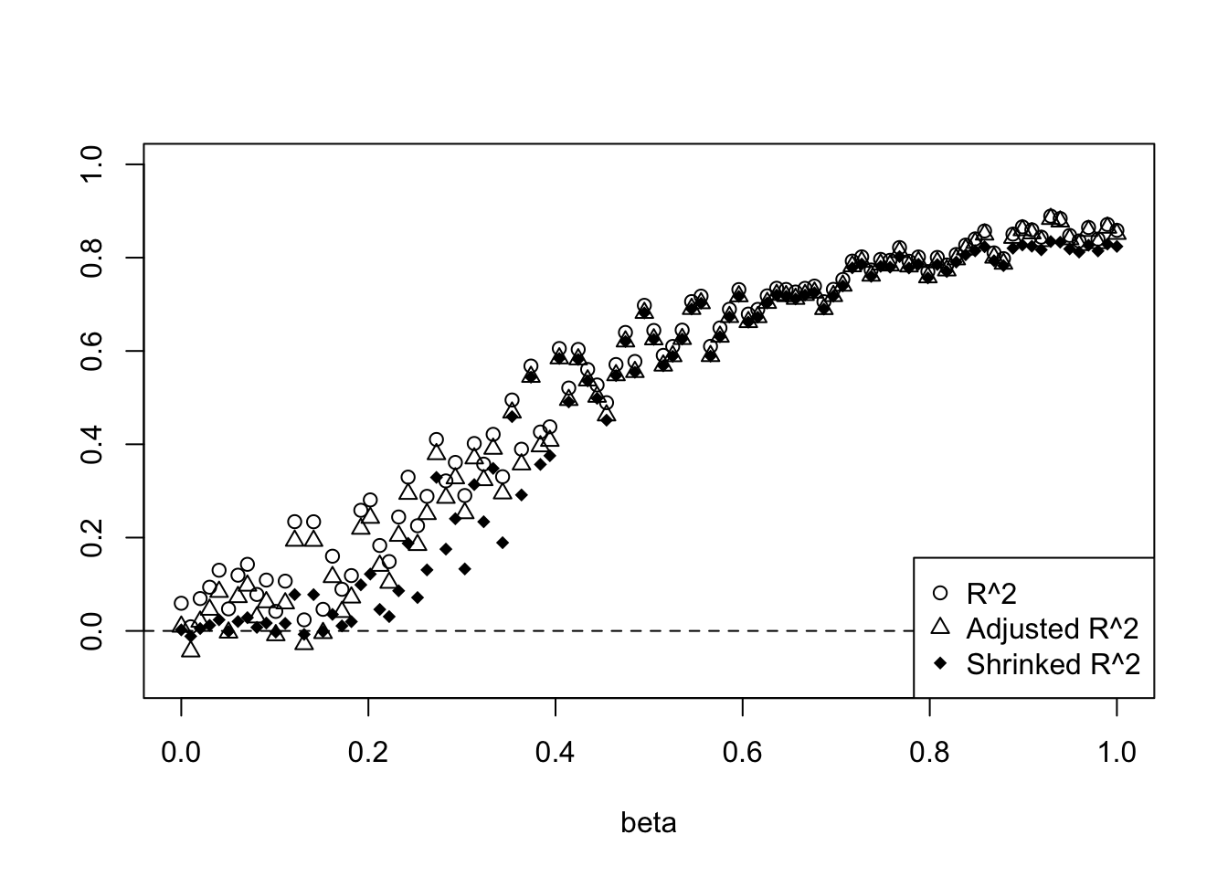
Expand here to see past versions of unnamed-chunk-1-1.png:
| Version | Author | Date |
|---|---|---|
| a17b894 | Dongyue Xie | 2019-01-16 |
plot(beta.list,R2,ylim=c(-0.1,1),main='',xlab='beta',ylab='',type='l')
lines(beta.list,R2a,col=2)
lines(beta.list,R2s,col=4)
abline(h=0,lty=2)
legend('bottomright',c('R^2','Adjusted R^2','Shrinked R^2'),lty=c(1,1,1),col=c(1,2,4))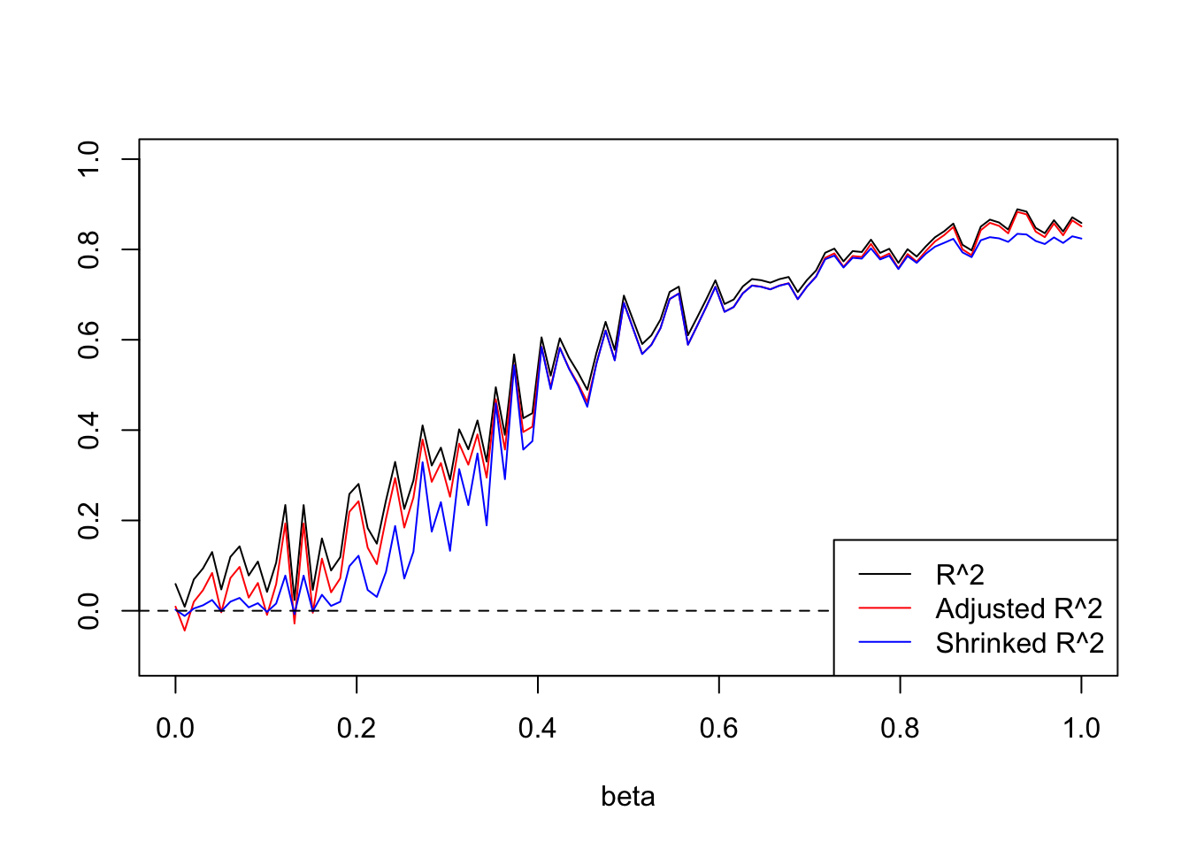
- First 50 \(\beta\)s are 0, last 50 \(\beta\)s range from 0 to 1. The other settings are the same as those in 1.
set.seed(1234)
n=100
p=5
R2=c()
R2a=c()
mset=c()
R2s=c()
beta.list=c(rep(0,50),seq(0,1,length.out = 50))
X=matrix(rnorm(n*(p)),n,p)
for (i in 1:length(beta.list)) {
  beta=rep(beta.list[i],p)
  y=X%*%beta+rnorm(n)
  datax=data.frame(X=X,y=y)
  mod=lm(y~X,datax)
  mod.sy=summary(mod)
  R2[i]=mod.sy$r.squared
  R2a[i]=mod.sy$adj.r.squared

  mst=sum((y-mean(y))^2)/(n-1)
  mse=sum((y-fitted(mod))^2)/(n-p-1)
  mset[i]=mse/mst

}

aa=ash(log(mset),1,lik=lik_logF(df1=n-p-1,df2=n-1))
R2s=1-exp(aa$result$PosteriorMean)

plot(R2,ylim=c(-0.1,1),main='',ylab='R^2')
lines(R2a,type='p',pch=2)
lines(R2s,type='p',pch=18)
abline(h=0,lty=2)
legend('bottomright',c('R^2','Adjusted R^2','Shrinked R^2'),pch=c(1,2,18))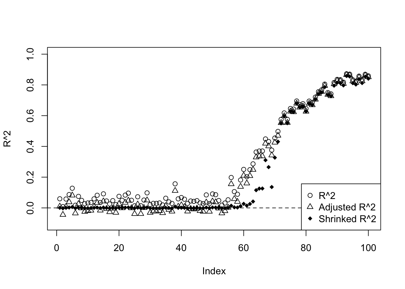
Expand here to see past versions of unnamed-chunk-2-1.png:
| Version | Author | Date |
|---|---|---|
| a17b894 | Dongyue Xie | 2019-01-16 |
plot(R2,ylim=c(-0.1,1),main='',ylab='R^2',type='l')
lines(R2a,col=2)
lines(R2s,col=4)
abline(h=0,lty=2)
legend('bottomright',c('R^2','Adjusted R^2','Shrinked R^2'),lty=c(1,1,1),col=c(1,2,4))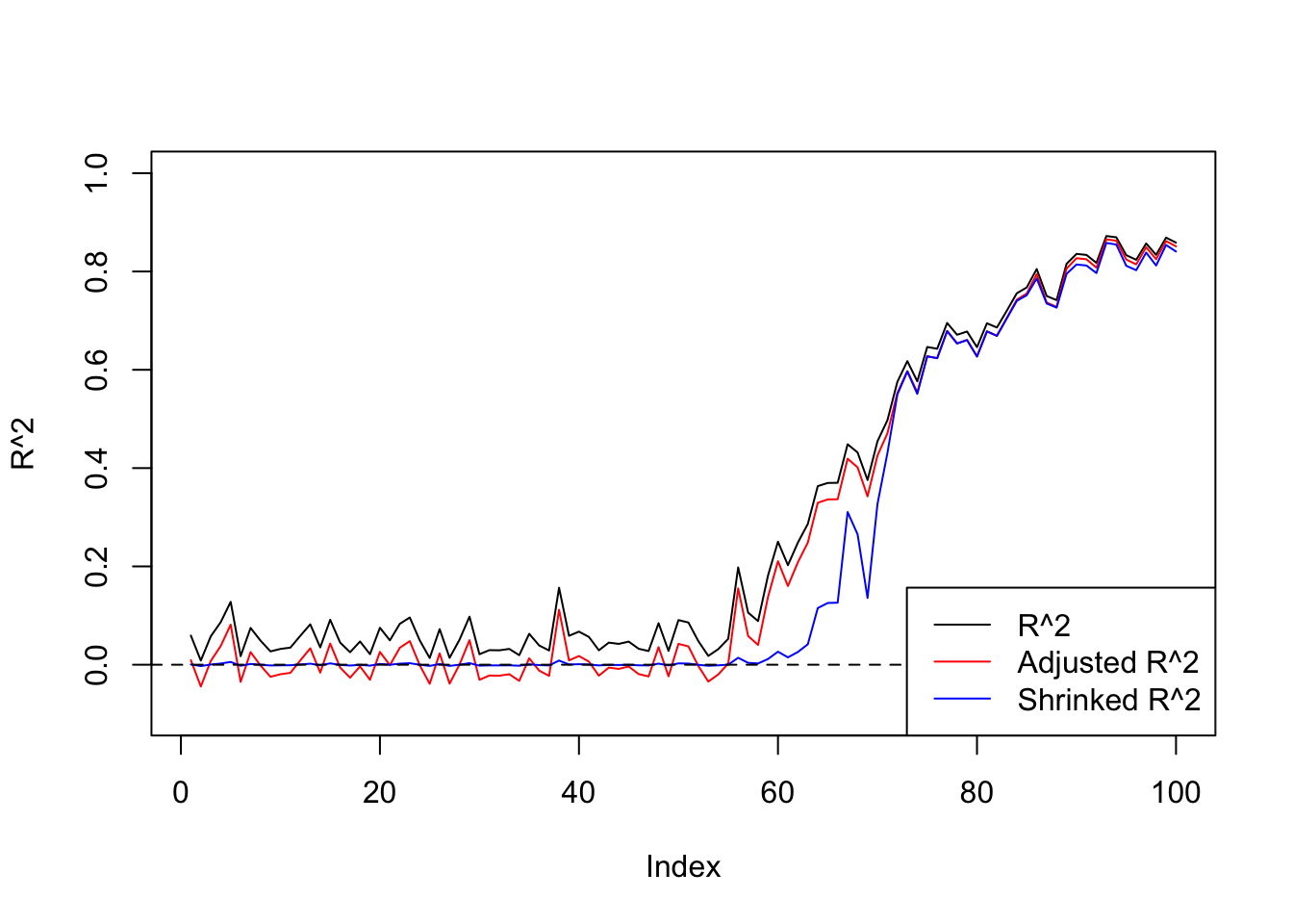
- Increase p to 20. The others are the same as those in 2.
set.seed(1234)
n=100
p=20
R2=c()
R2a=c()
mset=c()
R2s=c()
beta.list=c(rep(0,50),seq(0,1,length.out = 50))
X=matrix(rnorm(n*(p)),n,p)
for (i in 1:length(beta.list)) {
  beta=rep(beta.list[i],p)
  y=X%*%beta+rnorm(n)
  datax=data.frame(X=X,y=y)
  mod=lm(y~X,datax)
  mod.sy=summary(mod)
  R2[i]=mod.sy$r.squared
  R2a[i]=mod.sy$adj.r.squared

  mst=sum((y-mean(y))^2)/(n-1)
  mse=sum((y-fitted(mod))^2)/(n-p-1)
  mset[i]=mse/mst

}

aa=ash(log(mset),1,lik=lik_logF(df1=n-p-1,df2=n-1))
R2s=1-exp(aa$result$PosteriorMean)

plot(R2,ylim=c(-0.1,1),main='',ylab='R^2')
lines(R2a,type='p',pch=2)
lines(R2s,type='p',pch=18)
abline(h=0,lty=2)
legend('bottomright',c('R^2','Adjusted R^2','Shrinked R^2'),pch=c(1,2,18))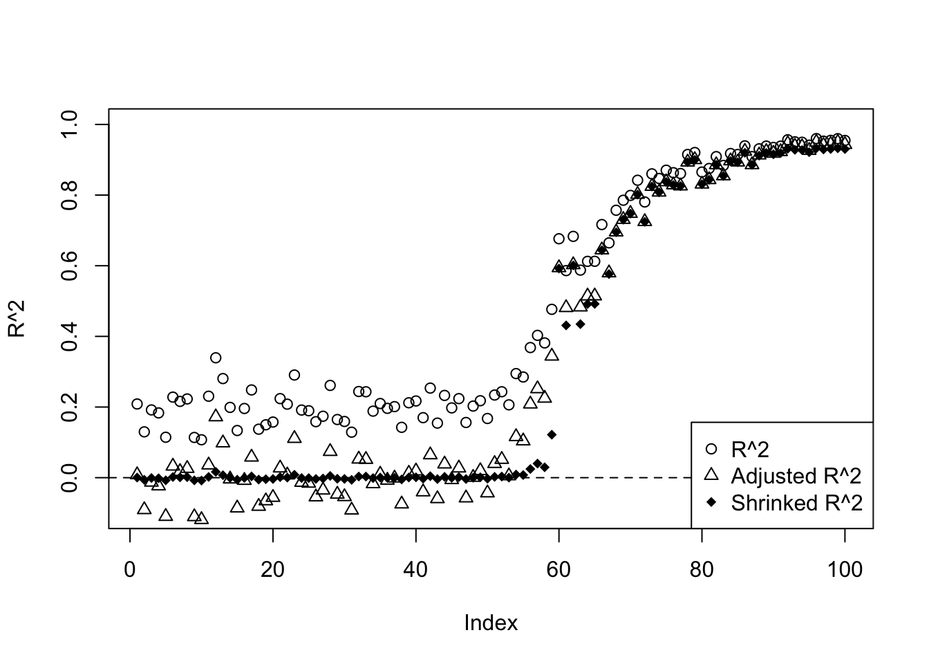
plot(R2,ylim=c(-0.1,1),main='',ylab='R^2',type='l')
lines(R2a,col=2)
lines(R2s,col=4)
abline(h=0,lty=2)
legend('bottomright',c('R^2','Adjusted R^2','Shrinked R^2'),lty=c(1,1,1),col=c(1,2,4))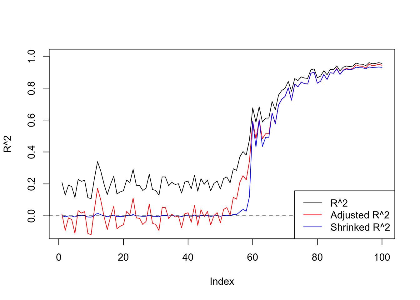
Facts might be useful
- Now try to relate \(R^2\) to F-statistics:
Define $ F^*=$, then \(F^*=\frac{SSR/(p-1)}{SSE/(n-p)}\sim F_{df_1=p-1,df_2=n-p}\) when \(\beta_1,...,\beta_{p-1}\) are 0. Otherwise, \(F^*\) follows non-central F distribution whose non-central parameter is \((X\beta)^T(H-\frac{11^T}{n})(X\beta)\).
- \(R=r_{y\hat y}\) where \(r\) is correlation coefficient.
Session information
sessionInfo()R version 3.5.1 (2018-07-02)
Platform: x86_64-apple-darwin15.6.0 (64-bit)
Running under: macOS High Sierra 10.13.6
Matrix products: default
BLAS: /Library/Frameworks/R.framework/Versions/3.5/Resources/lib/libRblas.0.dylib
LAPACK: /Library/Frameworks/R.framework/Versions/3.5/Resources/lib/libRlapack.dylib
locale:
[1] en_US.UTF-8/en_US.UTF-8/en_US.UTF-8/C/en_US.UTF-8/en_US.UTF-8
attached base packages:
[1] stats graphics grDevices utils datasets methods base
other attached packages:
[1] ashr_2.2-7
loaded via a namespace (and not attached):
[1] Rcpp_0.12.18 knitr_1.20 whisker_0.3-2
[4] magrittr_1.5 workflowr_1.1.1 REBayes_1.3
[7] MASS_7.3-50 pscl_1.5.2 doParallel_1.0.14
[10] SQUAREM_2017.10-1 lattice_0.20-35 foreach_1.4.4
[13] stringr_1.3.1 tools_3.5.1 parallel_3.5.1
[16] grid_3.5.1 R.oo_1.22.0 git2r_0.23.0
[19] htmltools_0.3.6 iterators_1.0.10 assertthat_0.2.0
[22] yaml_2.2.0 rprojroot_1.3-2 digest_0.6.17
[25] Matrix_1.2-14 codetools_0.2-15 R.utils_2.7.0
[28] evaluate_0.11 rmarkdown_1.10 stringi_1.2.4
[31] compiler_3.5.1 Rmosek_8.0.69 backports_1.1.2
[34] R.methodsS3_1.7.1 truncnorm_1.0-8 This reproducible R Markdown analysis was created with workflowr 1.1.1