10X Example
Last updated: 2018-08-30
workflowr checks: (Click a bullet for more information)-
✔ R Markdown file: up-to-date
Great! Since the R Markdown file has been committed to the Git repository, you know the exact version of the code that produced these results.
-
✔ Environment: empty
Great job! The global environment was empty. Objects defined in the global environment can affect the analysis in your R Markdown file in unknown ways. For reproduciblity it’s best to always run the code in an empty environment.
-
✔ Seed:
set.seed(20180618)The command
set.seed(20180618)was run prior to running the code in the R Markdown file. Setting a seed ensures that any results that rely on randomness, e.g. subsampling or permutations, are reproducible. -
✔ Session information: recorded
Great job! Recording the operating system, R version, and package versions is critical for reproducibility.
-
Great! You are using Git for version control. Tracking code development and connecting the code version to the results is critical for reproducibility. The version displayed above was the version of the Git repository at the time these results were generated.✔ Repository version: fa8da96
Note that you need to be careful to ensure that all relevant files for the analysis have been committed to Git prior to generating the results (you can usewflow_publishorwflow_git_commit). workflowr only checks the R Markdown file, but you know if there are other scripts or data files that it depends on. Below is the status of the Git repository when the results were generated:
Note that any generated files, e.g. HTML, png, CSS, etc., are not included in this status report because it is ok for generated content to have uncommitted changes.Ignored files: Ignored: .Rhistory Ignored: .Rproj.user/ Ignored: R/.Rhistory Ignored: analysis/.Rhistory Ignored: analysis/pipeline/.Rhistory Untracked files: Untracked: ..gif Untracked: .DS_Store Untracked: R/.DS_Store Untracked: R/myheatmap.R Untracked: analysis/.DS_Store Untracked: analysis/10x_heatmap.pdf Untracked: analysis/SLSL_marker_based_logcpm.pdf Untracked: analysis/biomarkers.R Untracked: analysis/cellref.pdf Untracked: analysis/consistency_check.R Untracked: analysis/dropseq_heatmap.pdf Untracked: analysis/dropseq_sc3_result.Rdata Untracked: analysis/dropseq_slsl1.Rdata Untracked: analysis/marker-based.pdf Untracked: analysis/normalization_test.R Untracked: analysis/pbmcheat.pdf Untracked: analysis/pbmcref.pdf Untracked: analysis/pipeline/0_dropseq/ Untracked: analysis/pipeline/1_10X/ Untracked: analysis/pipeline/2_zeisel/ Untracked: analysis/pipeline/3_smallsets/ Untracked: analysis/writeup/cite.log Untracked: analysis/writeup/paper.aux Untracked: analysis/writeup/paper.bbl Untracked: analysis/writeup/paper.blg Untracked: analysis/writeup/paper.log Untracked: analysis/writeup/paper.out Untracked: analysis/writeup/paper.synctex.gz Untracked: analysis/writeup/paper.tex Untracked: analysis/writeup/writeup.aux Untracked: analysis/writeup/writeup.bbl Untracked: analysis/writeup/writeup.blg Untracked: analysis/writeup/writeup.dvi Untracked: analysis/writeup/writeup.log Untracked: analysis/writeup/writeup.out Untracked: analysis/writeup/writeup.synctex.gz Untracked: analysis/writeup/writeup.tex Untracked: analysis/writeup/writeup2.aux Untracked: analysis/writeup/writeup2.bbl Untracked: analysis/writeup/writeup2.blg Untracked: analysis/writeup/writeup2.log Untracked: analysis/writeup/writeup2.out Untracked: analysis/writeup/writeup2.pdf Untracked: analysis/writeup/writeup2.synctex.gz Untracked: analysis/writeup/writeup2.tex Untracked: analysis/writeup/writeup3.aux Untracked: analysis/writeup/writeup3.log Untracked: analysis/writeup/writeup3.out Untracked: analysis/writeup/writeup3.synctex.gz Untracked: analysis/writeup/writeup3.tex Untracked: data/unnecessary_in_building/ Untracked: dropseq_heatmap.pdf Untracked: normalized_out_1.Rdata Untracked: not_normalized_out_1.Rdata Untracked: src/.gitignore Untracked: tutorial2.Rmd Unstaged changes: Modified: NAMESPACE Modified: R/RcppExports.R Modified: analysis/example_dropseq.Rmd Modified: analysis/pipeline/.DS_Store Modified: analysis/writeup/.DS_Store Modified: data/.DS_Store
Expand here to see past versions:
Read Data : PBMC 27K
Read data. Keep the gene names separately.
orig = readMM('data/unnecessary_in_building/pbmc3k/matrix.mtx')
orig_genenames = read.table('data/unnecessary_in_building/pbmc3k/genes.tsv',
                            stringsAsFactors = FALSE)
Quality Control and Cell Selections
Get summary of the cells. The function “cellFilter” removes abnormal cells based on the read counts. The arguments minGene and maxGene restrict the number of genes detected in each cell. In 10X and Drop-seq data, having lower limit of 500 and upper limit of 2000 are generally appropriate. The cells with greater than 2000 detected genes are likeliy to be doublets, and those with less than 500 have too many dropouts. The default values are -Inf and Inf, so users are recommended to inspect the histogram of gene counts and determine the bounds. The function also requires the gene names to discover the mito-genes. Cells with high mitochondrial read proportion can indicate apoptosis. The default is 0.1.
nGene = Matrix::colSums(orig > 0)
hist(nGene)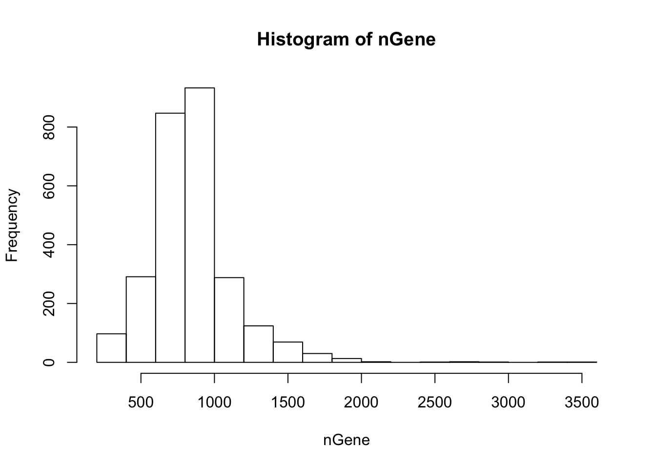
Expand here to see past versions of cell_filter-1.png:
| Version | Author | Date |
|---|---|---|
| f6c8902 | tk382 | 2018-08-29 |
summaryX = cellFilter(X = orig,
                      genenames = orig_genenames$V2,
                      minGene = 500,
                      maxGene = 2000,
                      maxMitoProp = 0.1)
tmpX = summaryX$X
nUMI = summaryX$nUMI
nGene = summaryX$nGene
percent.mito = summaryX$percent.mito
det.rate = summaryX$det.rate

par(mfrow = c(1,4))
boxplot(nUMI, main='nUMI');
boxplot(nGene, main='nGene');
boxplot(percent.mito, main='mitogene prop');
boxplot(det.rate, main='detection rate')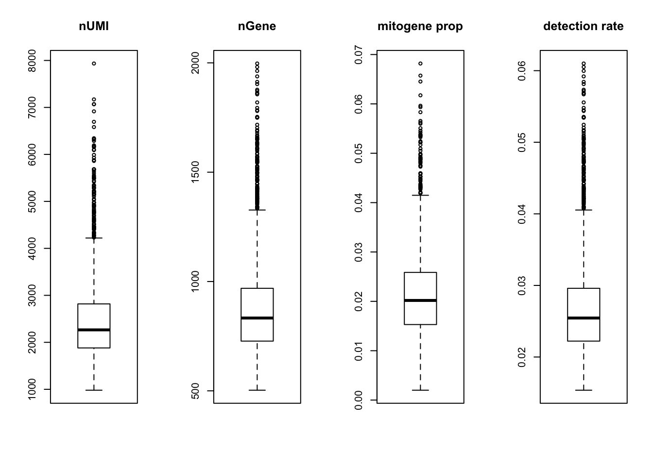
Expand here to see past versions of cell_filter-2.png:
| Version | Author | Date |
|---|---|---|
| f6c8902 | tk382 | 2018-08-29 |
Gene Filtering
Next find variable genes using normalized dispersion. First, remove the genes where counts are 0 in all the cells, so that we use genes with at least one UMI count detected in at least one cell are used. Then genes are placed into a number of bins (user’s choice in “bins” parameter in “dispersion” function, default is 20) based on their mean expression, and normalized dispersion is calculated as the absolute difference between dispersion and median dispersion of the expression mean, normalized by the median absolute deviation within each bin. (Grace Zheng et al., 2017)
X = tmpX[Matrix::rowSums(tmpX) > 0, ]
genenames = orig_genenames[Matrix::rowSums(tmpX) > 0, ]
disp = dispersion(X, bins = 20)
plot(disp$z ~ disp$genemeans,
     xlab = "mean expression",
     ylab = "normalized dispersion")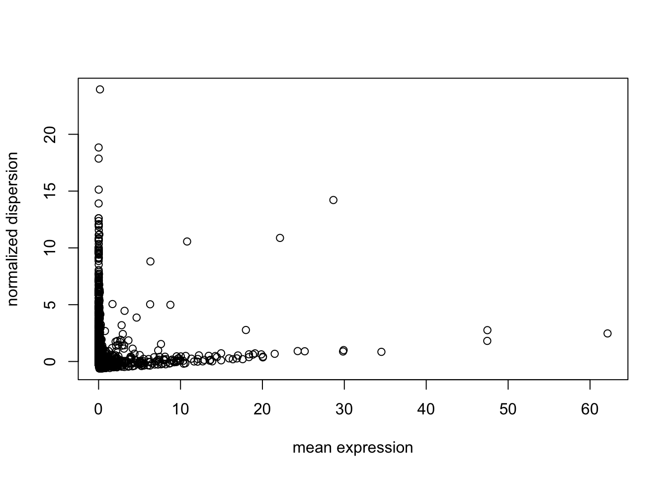
Expand here to see past versions of basic_gene_filtering-1.png:
| Version | Author | Date |
|---|---|---|
| f6c8902 | tk382 | 2018-08-29 |
select = which(abs(disp$z) > 1)
X = X[select, ]
genenames = genenames[select,]
UMI Normalization
Use quantile-normalization to make the distribution of each cell the same.
X = quantile_normalize(as.matrix(X))Correct Detection Rate
#take log
logX = as.matrix(log(X + 1))

#check dependency
out = correct_detection_rate(logX, det.rate)![]()
Expand here to see past versions of log_transform_and_det_correction-1.png:
| Version | Author | Date |
|---|---|---|
| f6c8902 | tk382 | 2018-08-29 |
#regress out
log.cpm = logX #not correct the detection rate (no strict linear pattern)
#if there is a pattern, log.cpm = out$residual
Dimension reduction and visualization
pc.base = irlba(log.cpm, 20)
tsne.base = Rtsne(pc.base$v[,1:10], dims=2, perplexity = 100, pca=FALSE)
rm(pc.base)
plot(tsne.base$Y, cex=0.5)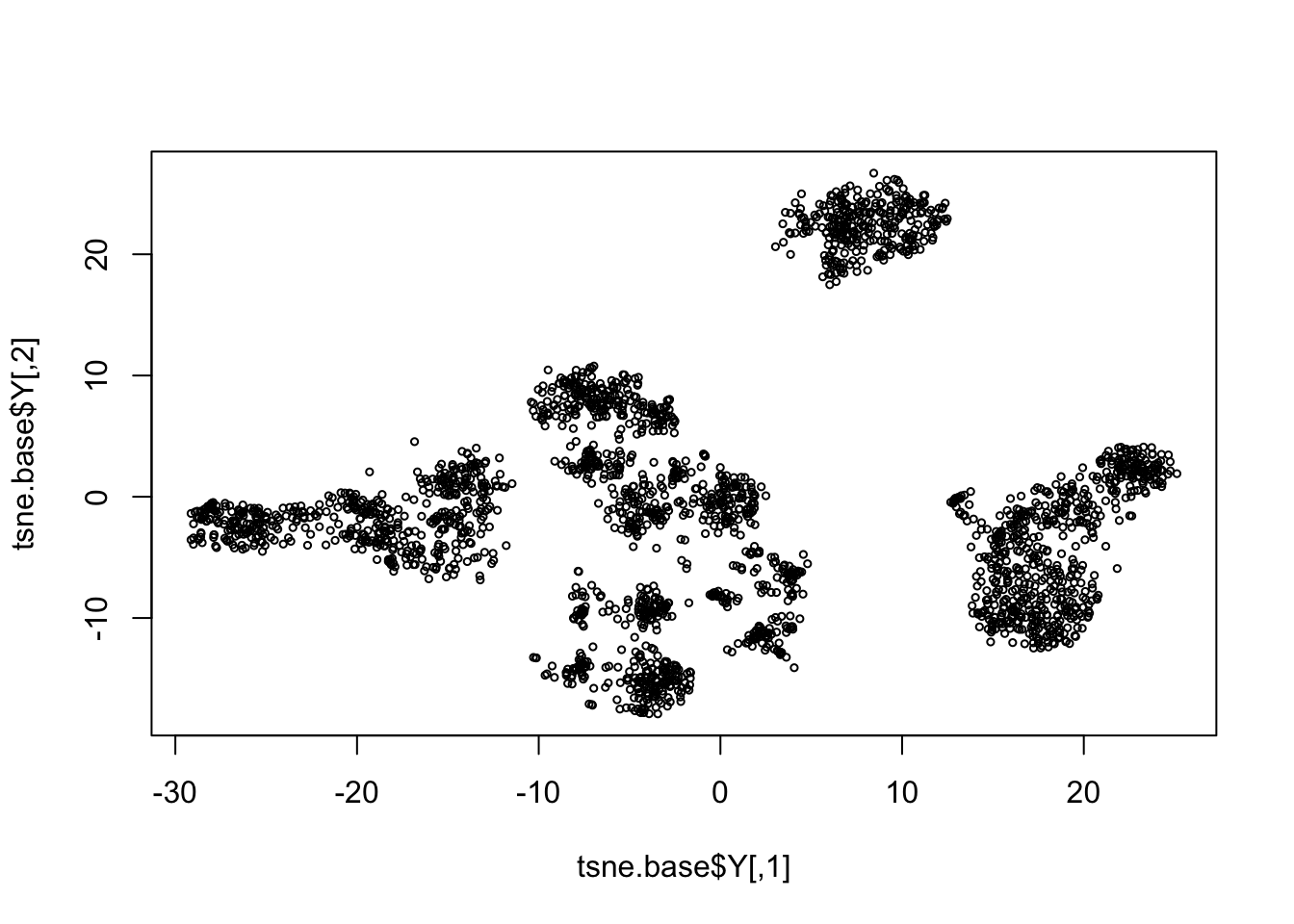
Expand here to see past versions of tsne-1.png:
| Version | Author | Date |
|---|---|---|
| f6c8902 | tk382 | 2018-08-29 |
Run SLSL
out = SLSL(log.cpm, log=FALSE,
           filter = FALSE,
           correct_detection_rate = FALSE,
           klist = c(200,250,300),
           sigmalist = c(1,1.5,2),
           kernel_type = "pearson",
           verbose=FALSE)
tab = table(out$result)
plot(tsne.base$Y, col=rainbow(7)[out$result],
     xlab = 'tsne1', ylab='tsne2', main="SLSL result", cex = 0.5)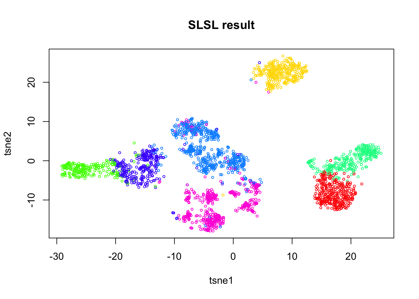
Expand here to see past versions of slsl-1.png:
| Version | Author | Date |
|---|---|---|
| f6c8902 | tk382 | 2018-08-29 |
S = as.matrix(out$S)
ind = sort(out$result, index.return=TRUE)$ix
palette.gr.marray <- colorRampPalette(c("ivory", "pink", "red", "brown"))(50)
heatmap.2(S[ind, ind],
          trace = "none",
          col = palette.gr.marray,
          Colv = F,
          Rowv = F,
          sepcolor = "gray",
          dendrogram = "none",
          labRow = NA,
          labCol = NA,
          key = F,
          breaks = seq(min(S), max(S),length=51),
          cexRow = 1,
          symbreaks = T)
Important Features
We use Kolgomorov-Smirov test to select some of the genes for the clusters not found in SC3 result to verify that our clustering result is based on real signals.
gene_selected_names = c('S100A4','B2M','LGALS1','S100A9','S100A8', 'LST1')
gene_selected = match(gene_selected_names, genenames$V2)
ind = gene_selected
df = data.frame(tsne1 = tsne.base$Y[,1], tsne2 = tsne.base$Y[,2],
                S100A4 = log.cpm[ind[1], ],
                B2M = log.cpm[ind[2], ],
                LGALS1 = log.cpm[ind[3],],
                S100A9 = log.cpm[ind[4], ],
                S100A8 = log.cpm[ind[5],],
                LST1 = log.cpm[ind[6], ])
g1 = ggplot(df, aes(x=tsne1, y=tsne2, col = S100A4)) + geom_point(size=0.1) +
  scale_colour_gradient(low="pink", high="black") + guides(color = FALSE) + ggtitle('S100A4')
g2 = ggplot(df, aes(x=tsne1, y=tsne2, col = B2M)) + geom_point(size=0.1) +
  scale_colour_gradient(low="pink", high="black") + guides(color = FALSE) + ggtitle('B2M')
g3 = ggplot(df, aes(x=tsne1, y=tsne2, col = LGALS1)) + geom_point(size=0.1) +
  scale_colour_gradient(low="pink", high="black") + guides(color = FALSE) + ggtitle('LGALS1')
g4 = ggplot(df, aes(x=tsne1, y=tsne2, col = S100A9)) + geom_point(size=0.1) +
  scale_colour_gradient(low="pink", high="black") + guides(color = FALSE) + ggtitle('S100A9')
g5 = ggplot(df, aes(x=tsne1, y=tsne2, col = S100A8)) + geom_point(size=0.1) +
  scale_colour_gradient(low="pink", high="black") + guides(color = FALSE) + ggtitle('S100A8')
g6 = ggplot(df, aes(x=tsne1, y=tsne2, col = LST1)) + geom_point(size=0.1) +
  scale_colour_gradient(low="pink", high="black") + guides(color = FALSE) + ggtitle('LST1')

grid.arrange(g1,g2,g3, g4,g5,g6,nrow=2)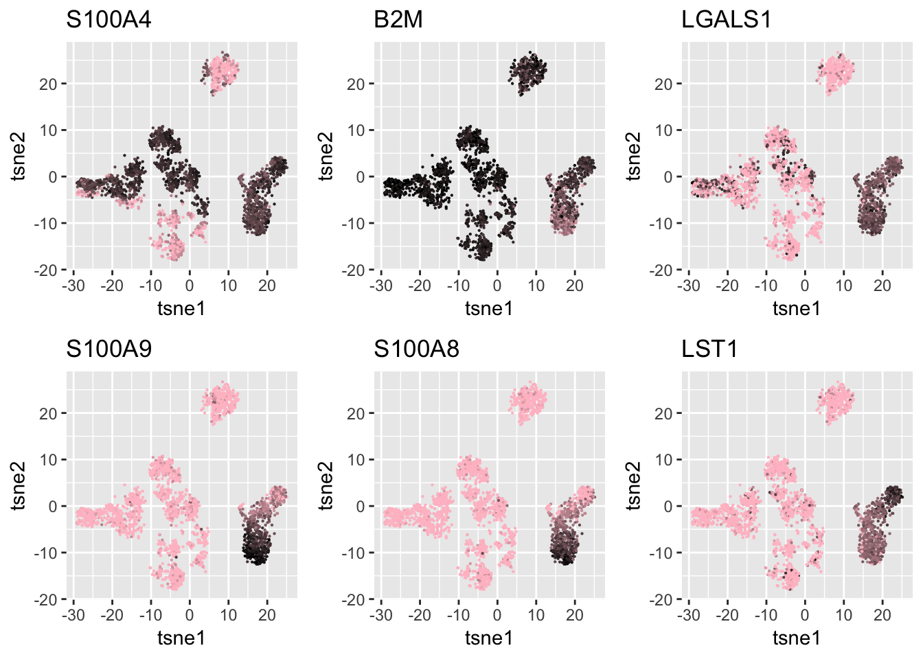
Expand here to see past versions of markers1-1.png:
| Version | Author | Date |
|---|---|---|
| f6c8902 | tk382 | 2018-08-29 |
Known Markers
I also check the markers provided in the past works about the same data set. The gene names used below are from either Seurat’s tutorial or the original 10X paper about PBMC cells Zheng et al.
#list comes from 10X paper and Seurat
ind = which(genenames$V2 %in% c('CD3D', 'CD8A', 'NKG7', 'FCER1A', 'CD16', 'S100A8',
                                     'MS4A1', 'GNLY', 'CD3E', 'CD14', 'FCGR3A',
                                     'LYZ','PPBP'))
genenames$V2[ind]
[1] "S100A8" "FCER1A" "GNLY" "PPBP" "LYZ" "NKG7" df = data.frame(tsne1 = tsne.base$Y[,1], tsne2 = tsne.base$Y[,2],
S100A8 = log.cpm[ind[1], ],
FCER1A = log.cpm[ind[2], ],
GNLY = log.cpm[ind[3], ],
PPBP = log.cpm[ind[4], ],
LYZ = log.cpm[ind[5], ],
NKG7 = log.cpm[ind[6], ])
g1 = ggplot(df, aes(x=tsne1, y=tsne2, col = S100A8)) + geom_point(size=0.1) +
scale_colour_gradient(low="pink", high="black") + guides(color = FALSE) + ggtitle('S100A8')
g2 = ggplot(df, aes(x=tsne1, y=tsne2, col = FCER1A)) + geom_point(size=0.1) +
scale_colour_gradient(low="pink", high="black") + guides(color = FALSE) + ggtitle('FCER1A')
g3 = ggplot(df, aes(x=tsne1, y=tsne2, col = GNLY)) + geom_point(size=0.1) +
scale_colour_gradient(low="pink", high="black") + guides(color = FALSE) + ggtitle('GNLY')
g4 = ggplot(df, aes(x=tsne1, y=tsne2, col = PPBP)) + geom_point(size=0.1) +
scale_colour_gradient(low="pink", high="black") + guides(color = FALSE) + ggtitle('PPBP')
g5 = ggplot(df, aes(x=tsne1, y=tsne2, col = LYZ)) + geom_point(size=0.1) + scale_colour_gradient(low="pink", high="black") + guides(color = FALSE) + ggtitle('LYZ')
g6 = ggplot(df, aes(x=tsne1, y=tsne2, col = NKG7)) + geom_point(size=0.1) + scale_colour_gradient(low="pink", high="black") + guides(color = FALSE) + ggtitle('NKG7')
grid.arrange(g1,g2,g3,g4,
g5,g6, nrow=2)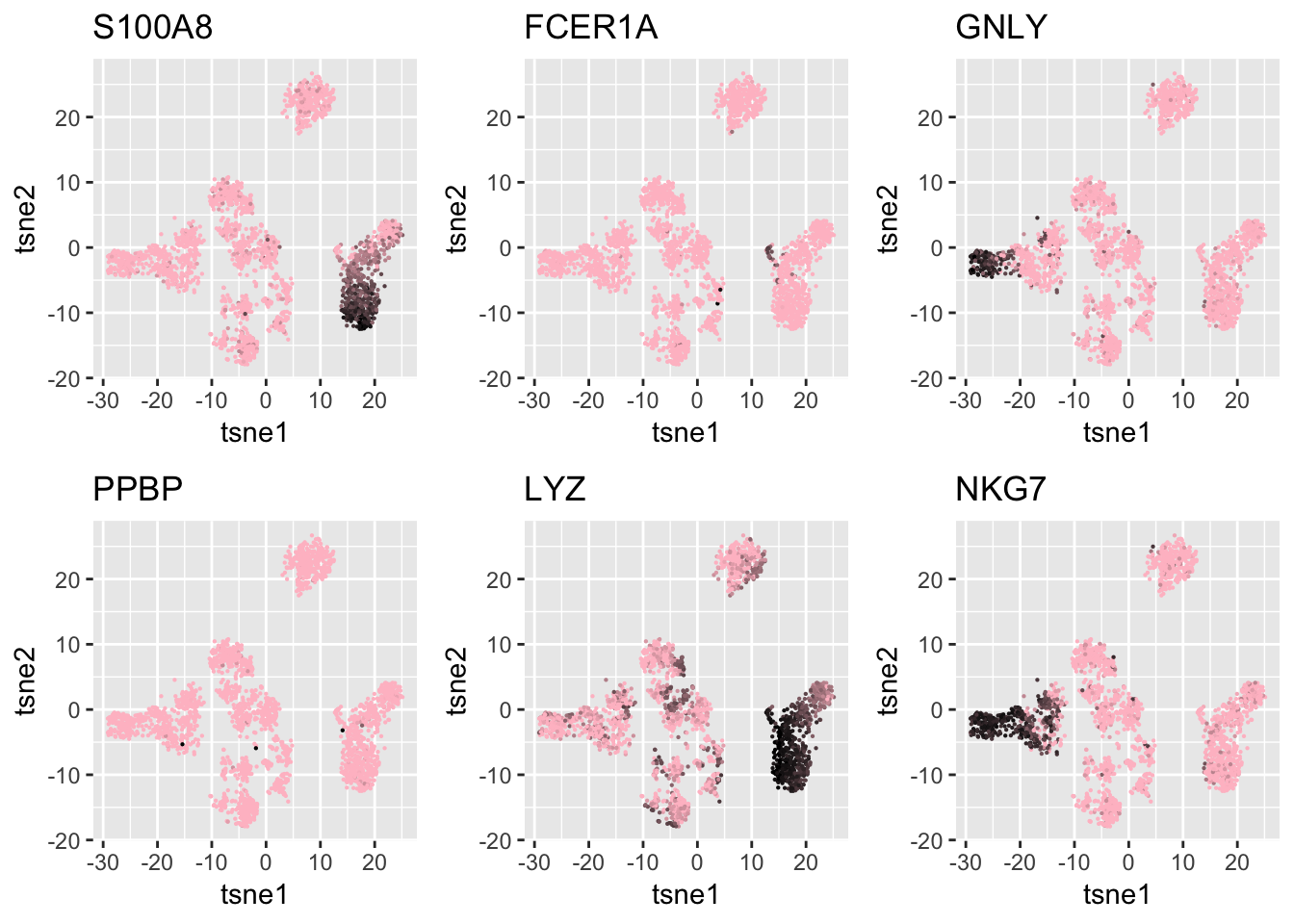
Expand here to see past versions of biomarkers-1.png:
| Version | Author | Date |
|---|---|---|
| f6c8902 | tk382 | 2018-08-29 |
Session information
sessionInfo()R version 3.5.1 (2018-07-02)
Platform: x86_64-apple-darwin15.6.0 (64-bit)
Running under: macOS Sierra 10.12.5
Matrix products: default
BLAS: /Library/Frameworks/R.framework/Versions/3.5/Resources/lib/libRblas.0.dylib
LAPACK: /Library/Frameworks/R.framework/Versions/3.5/Resources/lib/libRlapack.dylib
locale:
[1] en_US.UTF-8/en_US.UTF-8/en_US.UTF-8/C/en_US.UTF-8/en_US.UTF-8
attached base packages:
[1] parallel stats4 stats graphics grDevices utils datasets
[8] methods base
other attached packages:
[1] bindrcpp_0.2.2 gridExtra_2.3
[3] SC3_1.8.0 SingleCellExperiment_1.2.0
[5] SummarizedExperiment_1.10.1 DelayedArray_0.6.2
[7] BiocParallel_1.14.2 Biobase_2.40.0
[9] GenomicRanges_1.32.6 GenomeInfoDb_1.16.0
[11] IRanges_2.14.10 S4Vectors_0.18.3
[13] BiocGenerics_0.26.0 SCNoisyClustering_0.1.0
[15] plotly_4.8.0 gplots_3.0.1
[17] diceR_0.5.1 Rtsne_0.13
[19] igraph_1.2.2 scatterplot3d_0.3-41
[21] pracma_2.1.4 fossil_0.3.7
[23] shapefiles_0.7 foreign_0.8-71
[25] maps_3.3.0 sp_1.3-1
[27] caret_6.0-80 lattice_0.20-35
[29] reshape_0.8.7 dplyr_0.7.6
[31] quadprog_1.5-5 inline_0.3.15
[33] matrixStats_0.54.0 irlba_2.3.2
[35] Matrix_1.2-14 ggplot2_3.0.0
[37] MultiAssayExperiment_1.6.0
loaded via a namespace (and not attached):
[1] backports_1.1.2 workflowr_1.1.1
[3] plyr_1.8.4 lazyeval_0.2.1
[5] splines_3.5.1 digest_0.6.15
[7] foreach_1.4.4 htmltools_0.3.6
[9] gdata_2.18.0 magrittr_1.5
[11] cluster_2.0.7-1 doParallel_1.0.11
[13] ROCR_1.0-7 sfsmisc_1.1-2
[15] recipes_0.1.3 gower_0.1.2
[17] dimRed_0.1.0 R.utils_2.6.0
[19] colorspace_1.3-2 rrcov_1.4-4
[21] WriteXLS_4.0.0 crayon_1.3.4
[23] RCurl_1.95-4.11 jsonlite_1.5
[25] RcppArmadillo_0.8.600.0.0 bindr_0.1.1
[27] survival_2.42-6 iterators_1.0.10
[29] glue_1.3.0 DRR_0.0.3
[31] registry_0.5 gtable_0.2.0
[33] ipred_0.9-6 zlibbioc_1.26.0
[35] XVector_0.20.0 kernlab_0.9-26
[37] ddalpha_1.3.4 DEoptimR_1.0-8
[39] abind_1.4-5 scales_0.5.0
[41] mvtnorm_1.0-8 pheatmap_1.0.10
[43] rngtools_1.3.1 bibtex_0.4.2
[45] Rcpp_0.12.18 viridisLite_0.3.0
[47] xtable_1.8-2 magic_1.5-8
[49] mclust_5.4.1 lava_1.6.2
[51] prodlim_2018.04.18 htmlwidgets_1.2
[53] httr_1.3.1 RColorBrewer_1.1-2
[55] pkgconfig_2.0.1 R.methodsS3_1.7.1
[57] nnet_7.3-12 labeling_0.3
[59] later_0.7.3 tidyselect_0.2.4
[61] rlang_0.2.1 reshape2_1.4.3
[63] munsell_0.5.0 tools_3.5.1
[65] pls_2.6-0 broom_0.5.0
[67] evaluate_0.11 geometry_0.3-6
[69] stringr_1.3.1 yaml_2.2.0
[71] ModelMetrics_1.1.0 knitr_1.20
[73] robustbase_0.93-2 caTools_1.17.1.1
[75] purrr_0.2.5 nlme_3.1-137
[77] doRNG_1.7.1 mime_0.5
[79] whisker_0.3-2 R.oo_1.22.0
[81] RcppRoll_0.3.0 compiler_3.5.1
[83] e1071_1.7-0 tibble_1.4.2
[85] pcaPP_1.9-73 stringi_1.2.4
[87] pillar_1.3.0 data.table_1.11.4
[89] bitops_1.0-6 httpuv_1.4.5
[91] R6_2.2.2 promises_1.0.1
[93] KernSmooth_2.23-15 codetools_0.2-15
[95] MASS_7.3-50 gtools_3.8.1
[97] assertthat_0.2.0 CVST_0.2-2
[99] pkgmaker_0.27 rprojroot_1.3-2
[101] withr_2.1.2 GenomeInfoDbData_1.1.0
[103] grid_3.5.1 rpart_4.1-13
[105] timeDate_3043.102 tidyr_0.8.1
[107] class_7.3-14 rmarkdown_1.10
[109] git2r_0.23.0 shiny_1.1.0
[111] lubridate_1.7.4 This reproducible R Markdown analysis was created with workflowr 1.1.1