<!DOCTYPE html>

<html xmlns="http://www.w3.org/1999/xhtml">

<head>

<meta charset="utf-8" />
<meta http-equiv="Content-Type" content="text/html; charset=utf-8" />
<meta name="generator" content="pandoc" />


<title>Vector spatial data</title>

<script src="site_libs/jquery-1.12.4/jquery.min.js"></script>
<meta name="viewport" content="width=device-width, initial-scale=1" />
<link href="site_libs/bootstrap-3.3.5/css/cerulean.min.css" rel="stylesheet" />
<script src="site_libs/bootstrap-3.3.5/js/bootstrap.min.js"></script>
<script src="site_libs/bootstrap-3.3.5/shim/html5shiv.min.js"></script>
<script src="site_libs/bootstrap-3.3.5/shim/respond.min.js"></script>
<script src="site_libs/jqueryui-1.11.4/jquery-ui.min.js"></script>
<link href="site_libs/tocify-1.9.1/jquery.tocify.css" rel="stylesheet" />
<script src="site_libs/tocify-1.9.1/jquery.tocify.js"></script>
<script src="site_libs/navigation-1.1/tabsets.js"></script>
<script src="site_libs/htmlwidgets-1.2/htmlwidgets.js"></script>
<link href="site_libs/datatables-css-0.0.0/datatables-crosstalk.css" rel="stylesheet" />
<script src="site_libs/datatables-binding-0.4/datatables.js"></script>
<link href="site_libs/dt-core-1.10.16/css/jquery.dataTables.min.css" rel="stylesheet" />
<link href="site_libs/dt-core-1.10.16/css/jquery.dataTables.extra.css" rel="stylesheet" />
<script src="site_libs/dt-core-1.10.16/js/jquery.dataTables.min.js"></script>
<link href="site_libs/crosstalk-1.0.0/css/crosstalk.css" rel="stylesheet" />
<script src="site_libs/crosstalk-1.0.0/js/crosstalk.min.js"></script>
<link href="site_libs/font-awesome-5.0.13/css/fa-svg-with-js.css" rel="stylesheet" />
<script src="site_libs/font-awesome-5.0.13/js/fontawesome-all.min.js"></script>
<script src="site_libs/font-awesome-5.0.13/js/fa-v4-shims.min.js"></script>


<style type="text/css">code{white-space: pre;}</style>
<style type="text/css">
div.sourceCode { overflow-x: auto; }
table.sourceCode, tr.sourceCode, td.lineNumbers, td.sourceCode {
  margin: 0; padding: 0; vertical-align: baseline; border: none; }
table.sourceCode { width: 100%; line-height: 100%; background-color: #f8f8f8; }
td.lineNumbers { text-align: right; padding-right: 4px; padding-left: 4px; color: #aaaaaa; border-right: 1px solid #aaaaaa; }
td.sourceCode { padding-left: 5px; }
pre, code { background-color: #f8f8f8; }
code > span.kw { color: #204a87; font-weight: bold; } /* Keyword */
code > span.dt { color: #204a87; } /* DataType */
code > span.dv { color: #0000cf; } /* DecVal */
code > span.bn { color: #0000cf; } /* BaseN */
code > span.fl { color: #0000cf; } /* Float */
code > span.ch { color: #4e9a06; } /* Char */
code > span.st { color: #4e9a06; } /* String */
code > span.co { color: #8f5902; font-style: italic; } /* Comment */
code > span.ot { color: #8f5902; } /* Other */
code > span.al { color: #ef2929; } /* Alert */
code > span.fu { color: #000000; } /* Function */
code > span.er { color: #a40000; font-weight: bold; } /* Error */
code > span.wa { color: #8f5902; font-weight: bold; font-style: italic; } /* Warning */
code > span.cn { color: #000000; } /* Constant */
code > span.sc { color: #000000; } /* SpecialChar */
code > span.vs { color: #4e9a06; } /* VerbatimString */
code > span.ss { color: #4e9a06; } /* SpecialString */
code > span.im { } /* Import */
code > span.va { color: #000000; } /* Variable */
code > span.cf { color: #204a87; font-weight: bold; } /* ControlFlow */
code > span.op { color: #ce5c00; font-weight: bold; } /* Operator */
code > span.pp { color: #8f5902; font-style: italic; } /* Preprocessor */
code > span.ex { } /* Extension */
code > span.at { color: #c4a000; } /* Attribute */
code > span.do { color: #8f5902; font-weight: bold; font-style: italic; } /* Documentation */
code > span.an { color: #8f5902; font-weight: bold; font-style: italic; } /* Annotation */
code > span.cv { color: #8f5902; font-weight: bold; font-style: italic; } /* CommentVar */
code > span.in { color: #8f5902; font-weight: bold; font-style: italic; } /* Information */
</style>
<style type="text/css">
  pre:not([class]) {
    background-color: white;
  }
</style>


<style type="text/css">
h1 {
  font-size: 34px;
}
h1.title {
  font-size: 38px;
}
h2 {
  font-size: 30px;
}
h3 {
  font-size: 24px;
}
h4 {
  font-size: 18px;
}
h5 {
  font-size: 16px;
}
h6 {
  font-size: 12px;
}
.table th:not([align]) {
  text-align: left;
}
</style>


</head>

<body>

<style type = "text/css">
.main-container {
  max-width: 940px;
  margin-left: auto;
  margin-right: auto;
}
code {
  color: inherit;
  background-color: rgba(0, 0, 0, 0.04);
}
img {
  max-width:100%;
  height: auto;
}
.tabbed-pane {
  padding-top: 12px;
}
.html-widget {
  margin-bottom: 20px;
}
button.code-folding-btn:focus {
  outline: none;
}
</style>


<style type="text/css">
/* padding for bootstrap navbar */
body {
  padding-top: 51px;
  padding-bottom: 40px;
}
/* offset scroll position for anchor links (for fixed navbar)  */
.section h1 {
  padding-top: 56px;
  margin-top: -56px;
}

.section h2 {
  padding-top: 56px;
  margin-top: -56px;
}
.section h3 {
  padding-top: 56px;
  margin-top: -56px;
}
.section h4 {
  padding-top: 56px;
  margin-top: -56px;
}
.section h5 {
  padding-top: 56px;
  margin-top: -56px;
}
.section h6 {
  padding-top: 56px;
  margin-top: -56px;
}
</style>

<script>
// manage active state of menu based on current page
$(document).ready(function () {
  // active menu anchor
  href = window.location.pathname
  href = href.substr(href.lastIndexOf('/') + 1)
  if (href === "")
    href = "index.html";
  var menuAnchor = $('a[href="' + href + '"]');

  // mark it active
  menuAnchor.parent().addClass('active');

  // if it's got a parent navbar menu mark it active as well
  menuAnchor.closest('li.dropdown').addClass('active');
});
</script>


<div class="container-fluid main-container">

<!-- tabsets -->
<script>
$(document).ready(function () {
  window.buildTabsets("TOC");
});
</script>

<!-- code folding -->


<script>
$(document).ready(function ()  {

    // move toc-ignore selectors from section div to header
    $('div.section.toc-ignore')
        .removeClass('toc-ignore')
        .children('h1,h2,h3,h4,h5').addClass('toc-ignore');

    // establish options
    var options = {
      selectors: "h1,h2,h3",
      theme: "bootstrap3",
      context: '.toc-content',
      hashGenerator: function (text) {
        return text.replace(/[.\\/?&!#<>]/g, '').replace(/\s/g, '_').toLowerCase();
      },
      ignoreSelector: ".toc-ignore",
      scrollTo: 0
    };
    options.showAndHide = true;
    options.smoothScroll = true;

    // tocify
    var toc = $("#TOC").tocify(options).data("toc-tocify");
});
</script>

<style type="text/css">

#TOC {
  margin: 25px 0px 20px 0px;
}
@media (max-width: 768px) {
#TOC {
  position: relative;
  width: 100%;
}
}


.toc-content {
  padding-left: 30px;
  padding-right: 40px;
}

div.main-container {
  max-width: 1200px;
}

div.tocify {
  width: 20%;
  max-width: 260px;
  max-height: 85%;
}

@media (min-width: 768px) and (max-width: 991px) {
  div.tocify {
    width: 25%;
  }
}

@media (max-width: 767px) {
  div.tocify {
    width: 100%;
    max-width: none;
  }
}

.tocify ul, .tocify li {
  line-height: 20px;
}

.tocify-subheader .tocify-item {
  font-size: 0.90em;
  padding-left: 25px;
  text-indent: 0;
}

.tocify .list-group-item {
  border-radius: 0px;
}


</style>

<!-- setup 3col/9col grid for toc_float and main content  -->
<div class="row-fluid">
<div class="col-xs-12 col-sm-4 col-md-3">
<div id="TOC" class="tocify">
</div>
</div>

<div class="toc-content col-xs-12 col-sm-8 col-md-9">


<div class="navbar navbar-default  navbar-fixed-top" role="navigation">
  <div class="container">
    <div class="navbar-header">
      <button type="button" class="navbar-toggle collapsed" data-toggle="collapse" data-target="#navbar">
        <span class="icon-bar"></span>
        <span class="icon-bar"></span>
        <span class="icon-bar"></span>
      </button>
      <a class="navbar-brand" href="index.html">intro-r-gis</a>
    </div>
    <div id="navbar" class="navbar-collapse collapse">
      <ul class="nav navbar-nav">
        <li>
  <a href="index.html">Home</a>
</li>
<li>
  <a href="setup.html">Setup</a>
</li>
<li class="dropdown">
  <a href="#" class="dropdown-toggle" data-toggle="dropdown" role="button" aria-expanded="false">
    <span class="fa fa-gear"></span>
     
    Handouts
     
    <span class="caret"></span>
  </a>
  <ul class="dropdown-menu" role="menu">
    <li class="dropdown-header">Workshop Sections</li>
    <li>
      <a href="intro.html">Welcome</a>
    </li>
    <li>
      <a href="gis.html">Introduction to GIS</a>
    </li>
    <li>
      <a href="vector.html">Working with Vector Data</a>
    </li>
    <li>
      <a href="raster.html">Working with Raster Data</a>
    </li>
    <li class="divider"></li>
    <li>
      <a href="exercise_solutions.html">Exrecise solutions</a>
    </li>
  </ul>
</li>
      </ul>
      <ul class="nav navbar-nav navbar-right">
        <li>
  <a href="further_resources.html">Further Resources</a>
</li>
<li>
  <a href="https://github.com/annakrystalli/gis-workshop/archive/master.zip">Get Workshop Data</a>
</li>
<li>
  <a href="https://github.com/annakrystalli/intro-r-gis">
    <span class="fa fa-github"></span>
     
  </a>
</li>
      </ul>
    </div><!--/.nav-collapse -->
  </div><!--/.container -->
</div><!--/.navbar -->

<!-- Add a small amount of space between sections. -->
<style type="text/css">
div.section {
  padding-top: 12px;
}
</style>

<div class="fluid-row" id="header">


<h1 class="title toc-ignore">Vector spatial data</h1>

</div>


<p><strong>Last updated:</strong> 2018-09-05</p>
<strong>workflowr checks:</strong> <small>(Click a bullet for more information)</small>
<ul>
<li>
<p><details> <summary> <strong style="color:blue;">✔</strong> <strong>R Markdown file:</strong> up-to-date </summary></p>
<p>Great! Since the R Markdown file has been committed to the Git repository, you know the exact version of the code that produced these results.</p>
</details>
</li>
<li>
<p><details> <summary> <strong style="color:blue;">✔</strong> <strong>Environment:</strong> empty </summary></p>
<p>Great job! The global environment was empty. Objects defined in the global environment can affect the analysis in your R Markdown file in unknown ways. For reproduciblity it’s best to always run the code in an empty environment.</p>
</details>
</li>
<li>
<p><details> <summary> <strong style="color:blue;">✔</strong> <strong>Seed:</strong> <code>set.seed(20180820)</code> </summary></p>
<p>The command <code>set.seed(20180820)</code> was run prior to running the code in the R Markdown file. Setting a seed ensures that any results that rely on randomness, e.g. subsampling or permutations, are reproducible.</p>
</details>
</li>
<li>
<p><details> <summary> <strong style="color:blue;">✔</strong> <strong>Session information:</strong> recorded </summary></p>
<p>Great job! Recording the operating system, R version, and package versions is critical for reproducibility.</p>
</details>
</li>
<li>
<p><details> <summary> <strong style="color:blue;">✔</strong> <strong>Repository version:</strong> <a href="https://github.com/annakrystalli/intro-r-gis/tree/df988dcd2f505883a5474cb616b78edd885aa306" target="_blank">df988dc</a> </summary></p>
Great! You are using Git for version control. Tracking code development and connecting the code version to the results is critical for reproducibility. The version displayed above was the version of the Git repository at the time these results were generated. <br><br> Note that you need to be careful to ensure that all relevant files for the analysis have been committed to Git prior to generating the results (you can use <code>wflow_publish</code> or <code>wflow_git_commit</code>). workflowr only checks the R Markdown file, but you know if there are other scripts or data files that it depends on. Below is the status of the Git repository when the results were generated:
<pre><code>
Ignored files:
    Ignored:    .DS_Store
    Ignored:    .Rhistory
    Ignored:    .Rproj.user/
    Ignored:    analysis/.DS_Store
    Ignored:    analysis/assets/
    Ignored:    data-raw/
    Ignored:    data/csv/
    Ignored:    data/raster/
    Ignored:    data/sf/
    Ignored:    docs/.DS_Store

Untracked files:
    Untracked:  .Rbuildignore
    Untracked:  analysis/mapping.Rmd

Unstaged changes:
    Modified:   .gitignore
    Modified:   analysis/_site.yml

</code></pre>
Note that any generated files, e.g. HTML, png, CSS, etc., are not included in this status report because it is ok for generated content to have uncommitted changes. </details>
</li>
</ul>
<details> <summary> <small><strong>Expand here to see past versions:</strong></small> </summary>
<ul>
<table style="border-collapse:separate; border-spacing:5px;">
<thead>
<tr>
<th style="text-align:left;">
File
</th>
<th style="text-align:left;">
Version
</th>
<th style="text-align:left;">
Author
</th>
<th style="text-align:left;">
Date
</th>
<th style="text-align:left;">
Message
</th>
</tr>
</thead>
<tbody>
<tr>
<td style="text-align:left;">
Rmd
</td>
<td style="text-align:left;">
<a href="https://github.com/annakrystalli/intro-r-gis/blob/df988dcd2f505883a5474cb616b78edd885aa306/analysis/vector.Rmd" target="_blank">df988dc</a>
</td>
<td style="text-align:left;">
annakrystalli
</td>
<td style="text-align:left;">
2018-09-05
</td>
<td style="text-align:left;">
workflowr::wflow_publish(c(“analysis/vector.Rmd”))
</td>
</tr>
<tr>
<td style="text-align:left;">
html
</td>
<td style="text-align:left;">
<a href="https://cdn.rawgit.com/annakrystalli/intro-r-gis/2fff27badbcd342e17ecbf63caa6f698470886de/docs/vector.html" target="_blank">2fff27b</a>
</td>
<td style="text-align:left;">
annakrystalli
</td>
<td style="text-align:left;">
2018-09-05
</td>
<td style="text-align:left;">
Build site.
</td>
</tr>
<tr>
<td style="text-align:left;">
Rmd
</td>
<td style="text-align:left;">
<a href="https://github.com/annakrystalli/intro-r-gis/blob/fe9f11eb91e77232b5ae890b2de95d3184edc766/analysis/vector.Rmd" target="_blank">fe9f11e</a>
</td>
<td style="text-align:left;">
annakrystalli
</td>
<td style="text-align:left;">
2018-09-05
</td>
<td style="text-align:left;">
workflowr::wflow_publish(c(“analysis/vector.Rmd”))
</td>
</tr>
<tr>
<td style="text-align:left;">
html
</td>
<td style="text-align:left;">
<a href="https://cdn.rawgit.com/annakrystalli/intro-r-gis/ce5b92f3e0e2f729cb4d9156a2b9efd25a375d01/docs/vector.html" target="_blank">ce5b92f</a>
</td>
<td style="text-align:left;">
annakrystalli
</td>
<td style="text-align:left;">
2018-09-05
</td>
<td style="text-align:left;">
Build site.
</td>
</tr>
<tr>
<td style="text-align:left;">
Rmd
</td>
<td style="text-align:left;">
<a href="https://github.com/annakrystalli/intro-r-gis/blob/4e7deca4045636d6be4de90bcb54743c1c9e1212/analysis/vector.Rmd" target="_blank">4e7deca</a>
</td>
<td style="text-align:left;">
annakrystalli
</td>
<td style="text-align:left;">
2018-09-05
</td>
<td style="text-align:left;">
workflowr::wflow_publish(c(“analysis/vector.Rmd”))
</td>
</tr>
<tr>
<td style="text-align:left;">
html
</td>
<td style="text-align:left;">
<a href="https://cdn.rawgit.com/annakrystalli/intro-r-gis/88e2cb7dd0fb36fbd9df1593a44bef22187c0794/docs/vector.html" target="_blank">88e2cb7</a>
</td>
<td style="text-align:left;">
annakrystalli
</td>
<td style="text-align:left;">
2018-09-05
</td>
<td style="text-align:left;">
Build site.
</td>
</tr>
<tr>
<td style="text-align:left;">
html
</td>
<td style="text-align:left;">
<a href="https://cdn.rawgit.com/annakrystalli/intro-r-gis/2065eb46389f9e99d3bb57797c3b27f64a40849f/docs/vector.html" target="_blank">2065eb4</a>
</td>
<td style="text-align:left;">
annakrystalli
</td>
<td style="text-align:left;">
2018-09-04
</td>
<td style="text-align:left;">
Build site.
</td>
</tr>
<tr>
<td style="text-align:left;">
Rmd
</td>
<td style="text-align:left;">
<a href="https://github.com/annakrystalli/intro-r-gis/blob/82b5b1c092def80031f84fe934f91897103cad80/analysis/vector.Rmd" target="_blank">82b5b1c</a>
</td>
<td style="text-align:left;">
annakrystalli
</td>
<td style="text-align:left;">
2018-09-04
</td>
<td style="text-align:left;">
workflowr::wflow_publish(“analysis/vector.Rmd”)
</td>
</tr>
<tr>
<td style="text-align:left;">
html
</td>
<td style="text-align:left;">
<a href="https://cdn.rawgit.com/annakrystalli/intro-r-gis/48814f0796420500240638731346e1eb7b955c82/docs/vector.html" target="_blank">48814f0</a>
</td>
<td style="text-align:left;">
annakrystalli
</td>
<td style="text-align:left;">
2018-09-04
</td>
<td style="text-align:left;">
Build site.
</td>
</tr>
<tr>
<td style="text-align:left;">
html
</td>
<td style="text-align:left;">
<a href="https://cdn.rawgit.com/annakrystalli/intro-r-gis/8a975bc813c1c2196785cb9a30ec849bb50c60dd/docs/vector.html" target="_blank">8a975bc</a>
</td>
<td style="text-align:left;">
annakrystalli
</td>
<td style="text-align:left;">
2018-09-04
</td>
<td style="text-align:left;">
Build site.
</td>
</tr>
<tr>
<td style="text-align:left;">
Rmd
</td>
<td style="text-align:left;">
<a href="https://github.com/annakrystalli/intro-r-gis/blob/aae5895c3300bdc93507234fc95d61069e217bda/analysis/vector.Rmd" target="_blank">aae5895</a>
</td>
<td style="text-align:left;">
annakrystalli
</td>
<td style="text-align:left;">
2018-09-04
</td>
<td style="text-align:left;">
workflowr::wflow_publish(c(“analysis/vector.Rmd”))
</td>
</tr>
</tbody>
</table>
</ul>
<p></details></p>
<hr />
<div id="setup" class="section level2">
<h2>setup</h2>
<div id="open-notebook" class="section level3">
<h3>Open Notebook</h3>
<p>Open a new <strong>R Notebook</strong> to work in.</p>
<blockquote>
<p>File &gt; New File &gt; R Notebook</p>
</blockquote>
<p>Name (eg. <code>Vectors</code>) and save it</p>
</div>
<div id="load-libraries" class="section level3">
<h3>Load libraries</h3>
<p>Load the libraries we’ll be using for this section of the workshop</p>
<div class="sourceCode"><pre class="sourceCode r"><code class="sourceCode r"><span class="kw">library</span>(sf)
<span class="kw">library</span>(ggplot2)
<span class="kw">library</span>(dplyr)
<span class="kw">library</span>(spData)</code></pre></div>
</div>
</div>
<div id="vector-data" class="section level1">
<h1>Vector data</h1>
<p>Geographic vector data model is based on <strong>points</strong>, usually located within a coordinate reference system (CRS).</p>
<p>Most point geometries contain only two dimensions <span class="math inline">\(x\)</span> &amp; <span class="math inline">\(y\)</span> but 3 dimensional CRSs contain an additional <span class="math inline">\(z\)</span> value -&gt; height above sea level.</p>
<p>Coordinates consist of two numbers representing distance from an <strong>origin</strong> in the <span class="math inline">\(x\)</span> &amp; <span class="math inline">\(y\)</span> dimensions.</p>
<div id="simple-features" class="section level2">
<h2>simple features</h2>
<p>The <a href="https://en.wikipedia.org/wiki/Simple_Features"><strong>Simple Features data model</strong></a> is a widely supported model that underlies vector data structures in many GIS applications.</p>
<p>It is a <strong>hierarchical model</strong> that represents a <strong>wide range of geometry types</strong>.</p>
<ul>
<li><strong>single points</strong> -&gt; self-standing features (e.g. sampling location)</li>
<li>Points can be linked together to form more complex geometries:
<ul>
<li><strong>lines</strong></li>
<li><strong>polygons</strong></li>
</ul></li>
<li><strong>‘multi’ versions</strong> of each represent <strong>groups</strong> of features of the <strong>same type</strong> into a single feature.</li>
<li><strong>geometry collections</strong>, which can contain <strong>multiple geometry types</strong> in a single object.</li>
</ul>
<div class="figure">
<img src="https://geocompr.robinlovelace.net/figures/sf-classes.png" />

</div>
<p>*
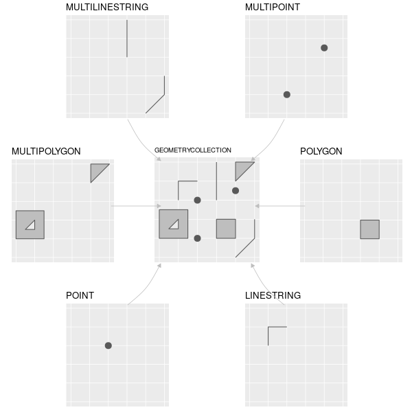
Figure 2.2: The subset of the Simple Features class hierarchy supported by sf. Image source: <a href="https://geocompr.robinlovelace.net/figures/sf-classes.png*" class="uri">https://geocompr.robinlovelace.net/figures/sf-classes.png*</a></p>
<div class="alert alert-success">
Of 68 geometry types supported by the specification, <strong>only 7 are used in the vast majority of geographic research</strong>
</div>
</div>
<div id="package-sf" class="section level2">
<h2>package <code>sf</code></h2>
<p><code>sf</code> is an R package <strong>providing a class system</strong> for geographic vector data using the <strong>simple features data model</strong>.</p>
<p>Supercedes and combines the functionality of three previously used packages: - <code>sp</code> for the class system, - <code>rgdal</code> for reading and writing data, - <code>rgeos</code> for spatial operations undertaken by GEOS in a single, cohesive whole.</p>
<div id="benefits-of-sf-vs-sp-classes" class="section level4">
<h4>Benefits of <code>sf</code> vs <code>sp</code> classes</h4>
<ul>
<li>Fast reading and writing of data</li>
<li>Enhanced plotting performance</li>
<li><code>sf</code> objects can be treated as data frames in most operations</li>
<li><code>sf</code> functions can be combined using the pipe (<code>%&gt;%</code>) operator and works well with the tidyverse collection of R packages</li>
<li><code>sf</code> function names are relatively consistent and intuitive (all begin with st_)</li>
<li>geometry a list in <code>geometry</code> column regardless of geometry type but can easily be transformed to a <code>Spatial</code> class used in <code>sp</code> using function <code>as_Spatial()</code>.</li>
</ul>
</div>
</div>
<div id="simple-feature-anatomy" class="section level2">
<h2>simple feature anatomy</h2>
<p>Simple feature objects are hierarchically organised as follows:</p>
<ul>
<li><code>sf</code>: <strong>simple feature</strong>, data.frame with <strong>spatial list-column</strong> (<code>geom</code> or <code>geometry</code>) as well as additional data associated with the spatial geometries.</li>
</ul>
<p><code>sfc</code>: <strong>simple feature column</strong>. A list-column containing <strong>multiple geometries</strong> + information about the coordinate reference system.</p>
<p><code>sfg</code>: <strong>simple feature geometry</strong>. a single simple feature geometry</p>
</div>
</div>
<div id="creating-sf-vector-data" class="section level1">
<h1>Creating <code>sf</code> vector data</h1>
<p><code>sf</code> provides a number of function for creating simple feature geometries, bringing multiple geometries together in a simple feature column.</p>
<div id="a-single-point-feature" class="section level3">
<h3>a single point feature</h3>
<p>To create <strong>single points</strong>, we can use function <code>sf::st_point()</code> and supply a <strong>vector of x &amp; y coordinates</strong> as argument <code>x</code></p>
<div class="sourceCode"><pre class="sourceCode r"><code class="sourceCode r"><span class="kw">st_point</span>(<span class="dt">x =</span> <span class="kw">c</span>(<span class="dv">0</span>,<span class="dv">0</span>))</code></pre></div>
</div>
<div id="multiple-point-feature" class="section level3">
<h3>multiple point feature</h3>
<p>For <strong>multiple points in a single geometry</strong>, we can use function <code>sf::st_multipoint()</code> and supply a <strong>two column numeric matrix</strong> with <strong>x &amp; y coordinates of points in rows</strong>.</p>
<div class="sourceCode"><pre class="sourceCode r"><code class="sourceCode r"><span class="kw">st_multipoint</span>(<span class="dt">x =</span> <span class="kw">matrix</span>(<span class="kw">c</span>(<span class="dv">0</span>, <span class="dv">0</span>, <span class="dv">1</span>, <span class="dv">0</span>), <span class="dt">ncol =</span> <span class="dv">2</span>, <span class="dt">byrow =</span> T))</code></pre></div>
<p>Let’s assign this to an object.</p>
<div class="sourceCode"><pre class="sourceCode r"><code class="sourceCode r">points &lt;-<span class="st"> </span><span class="kw">st_multipoint</span>(<span class="dt">x =</span> <span class="kw">matrix</span>(<span class="kw">c</span>(<span class="dv">0</span>, <span class="dv">0</span>, <span class="dv">2</span>, <span class="dv">0</span>), <span class="dt">ncol =</span> <span class="dv">2</span>, <span class="dt">byrow =</span> T))</code></pre></div>
<p>We can check the class of the points we just created:</p>
<div class="sourceCode"><pre class="sourceCode r"><code class="sourceCode r"><span class="kw">class</span>(points)</code></pre></div>
<pre><code>[1] &quot;XY&quot;         &quot;MULTIPOINT&quot; &quot;sfg&quot;       </code></pre>
<p>And we can also quickly plot geometries to inspect them:</p>
<div class="sourceCode"><pre class="sourceCode r"><code class="sourceCode r"><span class="kw">plot</span>(points)</code></pre></div>
<p><img src="figure/vector.Rmd/unnamed-chunk-6-1.png" width="672" style="display: block; margin: auto;" /></p>
<details> <summary><em>Expand here to see past versions of unnamed-chunk-6-1.png:</em></summary>
<table style="border-collapse:separate; border-spacing:5px;">
<thead>
<tr>
<th style="text-align:left;">
Version
</th>
<th style="text-align:left;">
Author
</th>
<th style="text-align:left;">
Date
</th>
</tr>
</thead>
<tbody>
<tr>
<td style="text-align:left;">
<a href="https://github.com/annakrystalli/intro-r-gis/blob/8a975bc813c1c2196785cb9a30ec849bb50c60dd/docs/figure/vector.Rmd/unnamed-chunk-6-1.png" target="_blank">8a975bc</a>
</td>
<td style="text-align:left;">
annakrystalli
</td>
<td style="text-align:left;">
2018-09-04
</td>
</tr>
</tbody>
</table>
<p></details></p>
</div>
<div id="line-feature" class="section level3">
<h3>line feature</h3>
<p>Similarly, we can create <strong>line features</strong> using function <code>sf::st_linestring()</code> and supplying a <strong>two column numeric matrix</strong> with <strong>x &amp; y coordinates of points in rows</strong>.</p>
<div class="sourceCode"><pre class="sourceCode r"><code class="sourceCode r">line &lt;-<span class="st"> </span><span class="kw">st_linestring</span>(<span class="dt">x =</span> <span class="kw">matrix</span>(<span class="kw">c</span>(<span class="op">-</span><span class="dv">1</span>, <span class="op">-</span><span class="dv">2</span>, <span class="op">-</span><span class="fl">0.5</span>, <span class="op">-</span><span class="dv">3</span>, <span class="fl">2.5</span>, <span class="op">-</span><span class="dv">3</span>, <span class="dv">3</span>, <span class="op">-</span><span class="dv">2</span>), 
                                 <span class="dt">ncol =</span> <span class="dv">2</span>, <span class="dt">byrow =</span> T))

line</code></pre></div>
<div class="sourceCode"><pre class="sourceCode r"><code class="sourceCode r"><span class="kw">plot</span>(line)</code></pre></div>
<p><img src="figure/vector.Rmd/unnamed-chunk-8-1.png" width="672" style="display: block; margin: auto;" /></p>
<details> <summary><em>
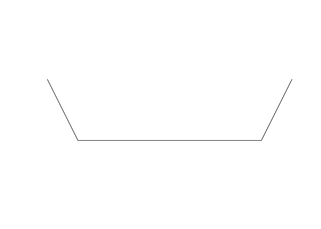
Expand here to see past versions of unnamed-chunk-8-1.png:</em></summary>
<table style="border-collapse:separate; border-spacing:5px;">
<thead>
<tr>
<th style="text-align:left;">
Version
</th>
<th style="text-align:left;">
Author
</th>
<th style="text-align:left;">
Date
</th>
</tr>
</thead>
<tbody>
<tr>
<td style="text-align:left;">
<a href="https://github.com/annakrystalli/intro-r-gis/blob/8a975bc813c1c2196785cb9a30ec849bb50c60dd/docs/figure/vector.Rmd/unnamed-chunk-8-1.png" target="_blank">8a975bc</a>
</td>
<td style="text-align:left;">
annakrystalli
</td>
<td style="text-align:left;">
2018-09-04
</td>
</tr>
</tbody>
</table>
<p></details></p>
</div>
<div id="combining-sfgs-into-an-sfc" class="section level3">
<h3>Combining <code>sfg</code>s into an <code>sfc</code></h3>
<p>We can then combine our geometries into an <strong>simple feature list-column</strong> (<code>sfc</code>).</p>
<div class="sourceCode"><pre class="sourceCode r"><code class="sourceCode r">sfc &lt;-<span class="st"> </span><span class="kw">st_sfc</span>(points, line)</code></pre></div>
<div class="sourceCode"><pre class="sourceCode r"><code class="sourceCode r"><span class="kw">class</span>(sfc)</code></pre></div>
<pre><code>[1] &quot;sfc_GEOMETRY&quot; &quot;sfc&quot;         </code></pre>
<div class="sourceCode"><pre class="sourceCode r"><code class="sourceCode r"><span class="kw">plot</span>(sfc)</code></pre></div>
<p><img src="figure/vector.Rmd/unnamed-chunk-11-1.png" width="672" style="display: block; margin: auto;" /></p>
<details> <summary><em>
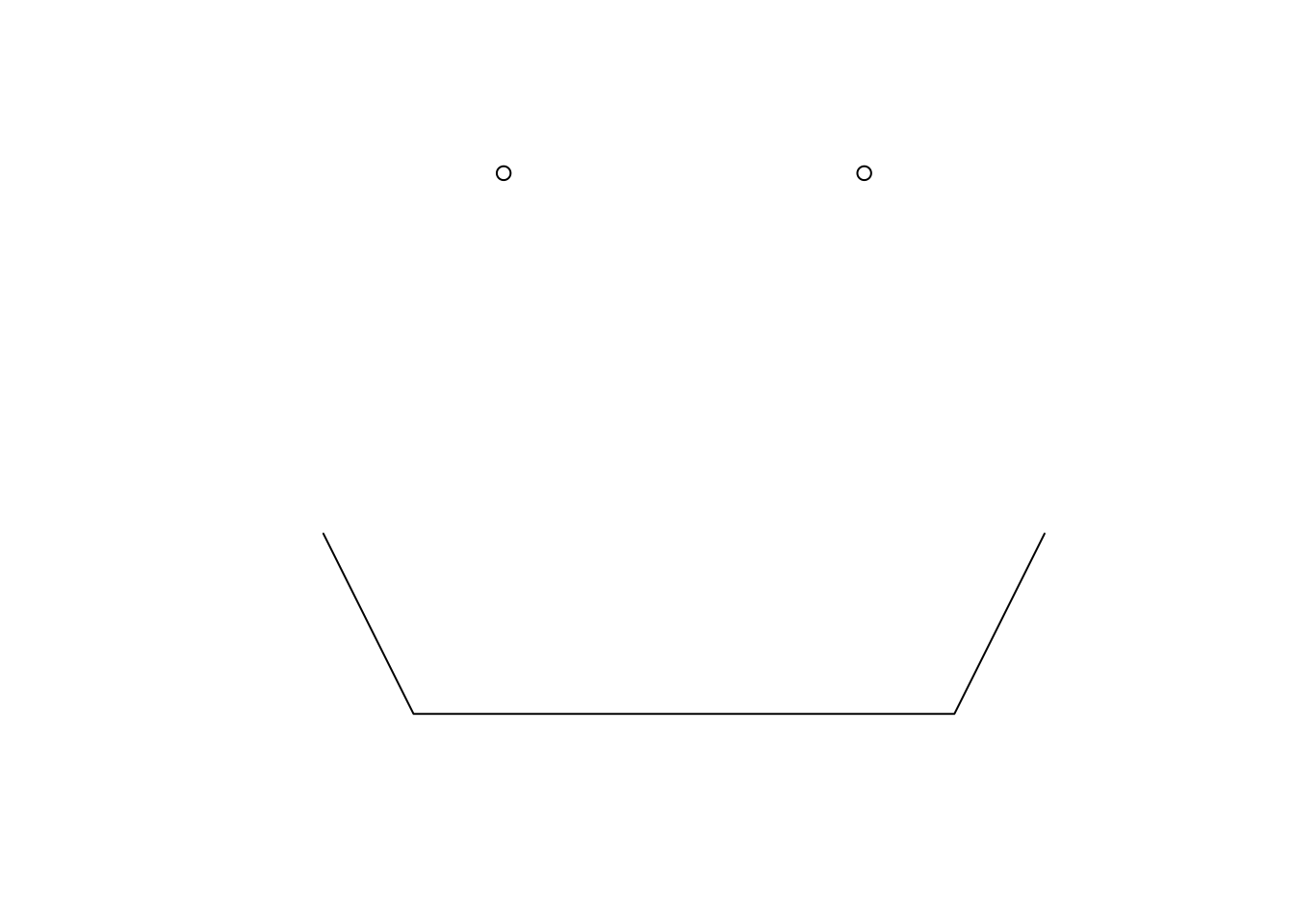
Expand here to see past versions of unnamed-chunk-11-1.png:</em></summary>
<table style="border-collapse:separate; border-spacing:5px;">
<thead>
<tr>
<th style="text-align:left;">
Version
</th>
<th style="text-align:left;">
Author
</th>
<th style="text-align:left;">
Date
</th>
</tr>
</thead>
<tbody>
<tr>
<td style="text-align:left;">
<a href="https://github.com/annakrystalli/intro-r-gis/blob/8a975bc813c1c2196785cb9a30ec849bb50c60dd/docs/figure/vector.Rmd/unnamed-chunk-11-1.png" target="_blank">8a975bc</a>
</td>
<td style="text-align:left;">
annakrystalli
</td>
<td style="text-align:left;">
2018-09-04
</td>
</tr>
</tbody>
</table>
<p></details></p>
</div>
<div id="creating-an-sf-and-adding-attribute-data" class="section level3">
<h3>Creating an <code>sf</code> and adding attribute data</h3>
<p>We can now add some attribute data, eg names for the shapes we created, and create a <strong>simple feature</strong> (<code>sf</code>).</p>
<div class="sourceCode"><pre class="sourceCode r"><code class="sourceCode r">sf &lt;-<span class="st"> </span><span class="kw">st_sf</span>(<span class="dt">shape =</span> <span class="kw">c</span>(<span class="st">&quot;eyes&quot;</span>, <span class="st">&quot;mouth&quot;</span>), <span class="dt">geom =</span> sfc)
sf</code></pre></div>
<pre><code>Simple feature collection with 2 features and 1 field
geometry type:  GEOMETRY
dimension:      XY
bbox:           xmin: -1 ymin: -3 xmax: 3 ymax: 0
epsg (SRID):    NA
proj4string:    NA
  shape                           geom
1  eyes          MULTIPOINT (0 0, 2 0)
2 mouth LINESTRING (-1 -2, -0.5 -3,...</code></pre>
<div class="sourceCode"><pre class="sourceCode r"><code class="sourceCode r"><span class="kw">class</span>(sf)</code></pre></div>
<pre><code>[1] &quot;sf&quot;         &quot;data.frame&quot;</code></pre>
<div class="sourceCode"><pre class="sourceCode r"><code class="sourceCode r"><span class="kw">plot</span>(sf)</code></pre></div>
<p><img src="figure/vector.Rmd/unnamed-chunk-14-1.png" width="672" style="display: block; margin: auto;" /></p>
<details> <summary><em>
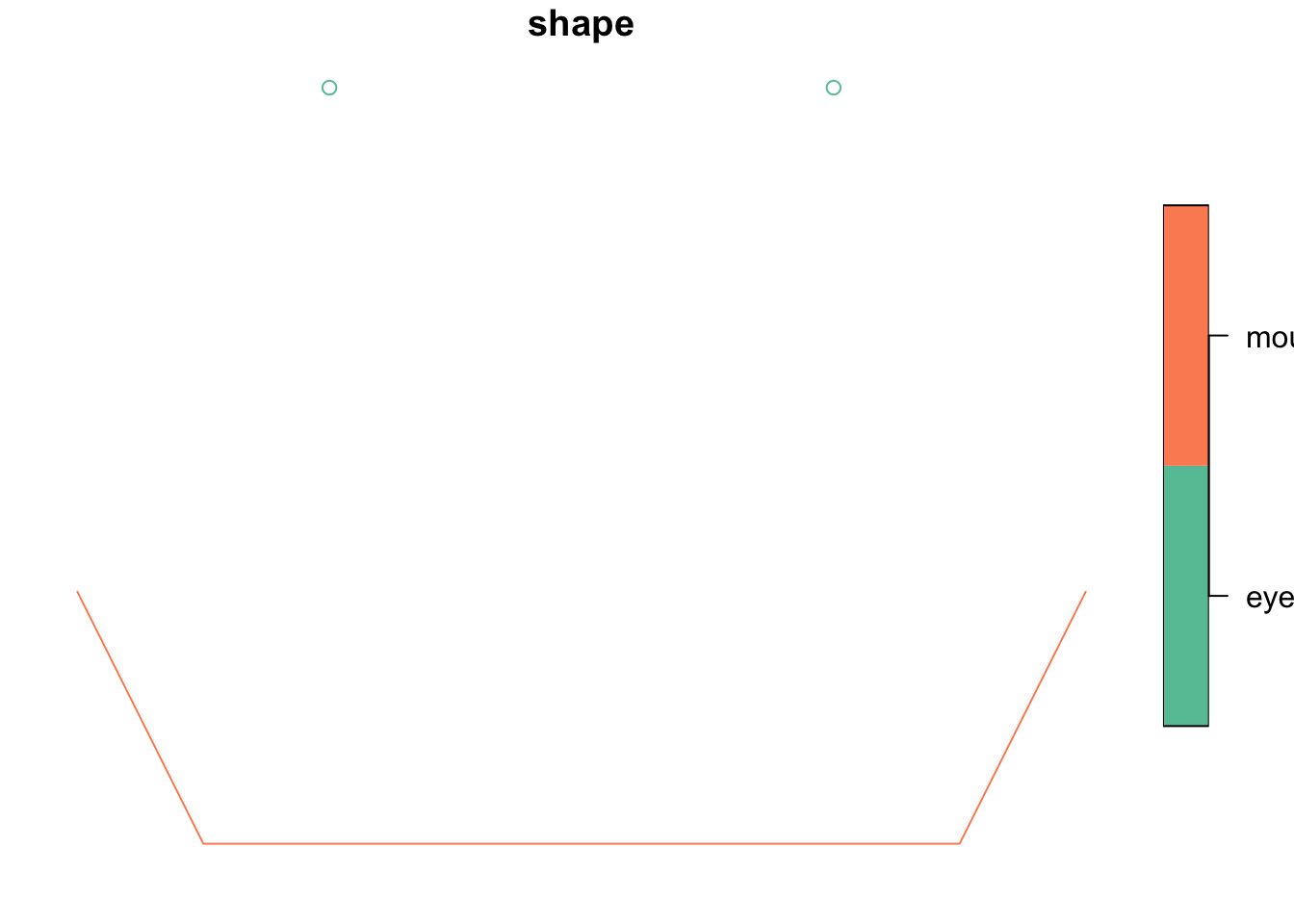
Expand here to see past versions of unnamed-chunk-14-1.png:</em></summary>
<table style="border-collapse:separate; border-spacing:5px;">
<thead>
<tr>
<th style="text-align:left;">
Version
</th>
<th style="text-align:left;">
Author
</th>
<th style="text-align:left;">
Date
</th>
</tr>
</thead>
<tbody>
<tr>
<td style="text-align:left;">
<a href="https://github.com/annakrystalli/intro-r-gis/blob/8a975bc813c1c2196785cb9a30ec849bb50c60dd/docs/figure/vector.Rmd/unnamed-chunk-14-1.png" target="_blank">8a975bc</a>
</td>
<td style="text-align:left;">
annakrystalli
</td>
<td style="text-align:left;">
2018-09-04
</td>
</tr>
</tbody>
</table>
<p></details></p>
</div>
<div id="exercise" class="section level3">
<h3>Exercise</h3>
<div id="add-a-nose" class="section level4">
<h4>1) add a nose!</h4>
<p>Create a nose geometry, combine all the shapes into a single <code>sf</code> and then plot the face.</p>
</div>
</div>
</div>
<div id="working-with-sf-vector-data" class="section level1">
<h1>Working with <code>sf</code> vector data</h1>
<div id="world-dataset-in-pkg-spdata" class="section level2">
<h2><code>world</code> dataset in pkg <code>spData</code></h2>
<p>Package <a href="https://github.com/Nowosad/spData"><code>spData</code></a> provides spatial datasets in a variety of formats, including a number of <code>sf</code> data.</p>
<p>One of these is the <code>world</code> data set, containing the current boundaries of countries and including additional demographic, geographic <strong>attribute</strong> data</p>
<div class="sourceCode"><pre class="sourceCode r"><code class="sourceCode r"><span class="kw">library</span>(spData)</code></pre></div>
<div class="sourceCode"><pre class="sourceCode r"><code class="sourceCode r">world</code></pre></div>
<pre><code>Simple feature collection with 177 features and 10 fields
geometry type:  MULTIPOLYGON
dimension:      XY
bbox:           xmin: -180 ymin: -90 xmax: 180 ymax: 83.64513
epsg (SRID):    4326
proj4string:    +proj=longlat +datum=WGS84 +no_defs
First 10 features:
   iso_a2        name_long     continent region_un          subregion
1      FJ             Fiji       Oceania   Oceania          Melanesia
2      TZ         Tanzania        Africa    Africa     Eastern Africa
3      EH   Western Sahara        Africa    Africa    Northern Africa
4      CA           Canada North America  Americas   Northern America
5      US    United States North America  Americas   Northern America
6      KZ       Kazakhstan          Asia      Asia       Central Asia
7      UZ       Uzbekistan          Asia      Asia       Central Asia
8      PG Papua New Guinea       Oceania   Oceania          Melanesia
9      ID        Indonesia          Asia      Asia South-Eastern Asia
10     AR        Argentina South America  Americas      South America
                type    area_km2       pop  lifeExp gdpPercap
1  Sovereign country    19289.97    885806 69.96000  8222.254
2  Sovereign country   932745.79  52234869 64.16300  2402.099
3      Indeterminate    96270.60        NA       NA        NA
4  Sovereign country 10036042.98  35535348 81.95305 43079.143
5            Country  9510743.74 318622525 78.84146 51921.985
6  Sovereign country  2729810.51  17288285 71.62000 23587.338
7  Sovereign country   461410.26  30757700 71.03900  5370.866
8  Sovereign country   464520.07   7755785 65.23000  3709.082
9  Sovereign country  1819251.33 255131116 68.85600 10003.089
10 Sovereign country  2784468.59  42981515 76.25200 18797.548
                             geom
1  MULTIPOLYGON (((180 -16.067...
2  MULTIPOLYGON (((33.90371 -0...
3  MULTIPOLYGON (((-8.66559 27...
4  MULTIPOLYGON (((-122.84 49,...
5  MULTIPOLYGON (((-122.84 49,...
6  MULTIPOLYGON (((87.35997 49...
7  MULTIPOLYGON (((55.96819 41...
8  MULTIPOLYGON (((141.0002 -2...
9  MULTIPOLYGON (((141.0002 -2...
10 MULTIPOLYGON (((-68.63401 -...</code></pre>
<p>Country polygons from the <code>world</code> dataset</p>
<p>We can get more information on the data containing through r help</p>
<div class="sourceCode"><pre class="sourceCode r"><code class="sourceCode r">?world</code></pre></div>
</div>
<div id="manipulating-sf-objects" class="section level2">
<h2>Manipulating <code>sf</code> objects</h2>
<p>As discussed the data is effectively a <code>data.frame</code>, with an additional <code>geom</code> column containing the geographic data. As such it can be manipulated as any other data.frame.</p>
<div id="getting-attribute-information" class="section level3">
<h3>getting attribute information</h3>
<div class="sourceCode"><pre class="sourceCode r"><code class="sourceCode r"><span class="kw">names</span>(world)</code></pre></div>
<pre><code> [1] &quot;iso_a2&quot;    &quot;name_long&quot; &quot;continent&quot; &quot;region_un&quot; &quot;subregion&quot;
 [6] &quot;type&quot;      &quot;area_km2&quot;  &quot;pop&quot;       &quot;lifeExp&quot;   &quot;gdpPercap&quot;
[11] &quot;geom&quot;     </code></pre>
</div>
<div id="indexing" class="section level3">
<h3>indexing</h3>
<p>We can index <code>sf</code> objects like any other data.frame.</p>
<p>E.g. we can index columns using the <code>$</code> notation:</p>
<div class="sourceCode"><pre class="sourceCode r"><code class="sourceCode r">world<span class="op">$</span>iso_a2</code></pre></div>
<pre><code>  [1] FJ   TZ   EH   CA   US   KZ   UZ   PG   ID   AR   CL   CD   SO   KE  
 [15] SD   TD   HT   DO   RU   BS   FK   &lt;NA&gt; GL   TF   TL   ZA   LS   MX  
 [29] UY   BR   BO   PE   CO   PA   CR   NI   HN   SV   GT   BZ   VE   GY  
 [43] SR   &lt;NA&gt; EC   PR   JM   CU   ZW   BW   NA   SN   ML   MR   BJ   NE  
 [57] NG   CM   TG   GH   CI   GN   GW   LR   SL   BF   CF   CG   GA   GQ  
 [71] ZM   MW   MZ   SZ   AO   BI   IL   LB   MG   PS   GM   TN   DZ   JO  
 [85] AE   QA   KW   IQ   OM   VU   KH   TH   LA   MM   VN   KP   KR   MN  
 [99] IN   BD   BT   NP   PK   AF   TJ   KG   TM   IR   SY   AM   SE   BY  
[113] UA   PL   AT   HU   MD   RO   LT   LV   EE   DE   BG   GR   TR   AL  
[127] HR   CH   LU   BE   NL   PT   ES   IE   NC   SB   NZ   AU   LK   CN  
[141] TW   IT   DK   GB   IS   AZ   GE   PH   MY   BN   SI   FI   SK   CZ  
[155] ER   JP   PY   YE   SA   AQ   &lt;NA&gt; CY   MA   EG   LY   ET   DJ   &lt;NA&gt;
[169] UG   RW   BA   MK   RS   ME   XK   TT   SS  
173 Levels: AE AF AL AM AO AQ AR AT AU AZ BA BD BE BF BG BI BJ BN BO ... ZW</code></pre>
<p>Or by using <code>[,]</code> indexing, in this case, by supplying a vector of column names to the second argument of the square brackets.</p>
<div class="sourceCode"><pre class="sourceCode r"><code class="sourceCode r">world[, <span class="kw">c</span>(<span class="st">&quot;iso_a2&quot;</span>, <span class="st">&quot;name_long&quot;</span>)]</code></pre></div>
<pre><code>Simple feature collection with 177 features and 2 fields
geometry type:  MULTIPOLYGON
dimension:      XY
bbox:           xmin: -180 ymin: -90 xmax: 180 ymax: 83.64513
epsg (SRID):    4326
proj4string:    +proj=longlat +datum=WGS84 +no_defs
First 10 features:
   iso_a2        name_long                           geom
1      FJ             Fiji MULTIPOLYGON (((180 -16.067...
2      TZ         Tanzania MULTIPOLYGON (((33.90371 -0...
3      EH   Western Sahara MULTIPOLYGON (((-8.66559 27...
4      CA           Canada MULTIPOLYGON (((-122.84 49,...
5      US    United States MULTIPOLYGON (((-122.84 49,...
6      KZ       Kazakhstan MULTIPOLYGON (((87.35997 49...
7      UZ       Uzbekistan MULTIPOLYGON (((55.96819 41...
8      PG Papua New Guinea MULTIPOLYGON (((141.0002 -2...
9      ID        Indonesia MULTIPOLYGON (((141.0002 -2...
10     AR        Argentina MULTIPOLYGON (((-68.63401 -...</code></pre>
<p>Note that although we selected only two columns, the <code>geom</code> column is still retained.</p>
<p>And we can index rows by supplying eg the row number(s) required to the first argument of the square brackets.</p>
<div class="sourceCode"><pre class="sourceCode r"><code class="sourceCode r">world[<span class="dv">1</span>,]</code></pre></div>
<pre><code>Simple feature collection with 1 feature and 10 fields
geometry type:  MULTIPOLYGON
dimension:      XY
bbox:           xmin: -180 ymin: -18.28799 xmax: 180 ymax: -16.02088
epsg (SRID):    4326
proj4string:    +proj=longlat +datum=WGS84 +no_defs
  iso_a2 name_long continent region_un subregion              type
1     FJ      Fiji   Oceania   Oceania Melanesia Sovereign country
  area_km2    pop lifeExp gdpPercap                           geom
1 19289.97 885806   69.96  8222.254 MULTIPOLYGON (((180 -16.067...</code></pre>
</div>
<div id="dplyr-functions-and-piping" class="section level3">
<h3><code>dplyr</code> functions and piping</h3>
<p>But even nicer is that we can use <code>dplyr</code> functions with <code>sf</code>s. Especially exciting is the <strong>ability to set up pipelines using the <code>dplyr</code> pipe (<code>%&gt;%</code>).</strong></p>
</div>
<div id="selecting" class="section level3">
<h3>selecting</h3>
<p>We can pipe the <code>spData::world</code> <code>sf</code> into function <code>dplyr::select()</code> to select specific columns. Note that in <code>dplyr</code> functions, you can use column names <strong>bare</strong> (ie without <code>&quot;...&quot;</code>).</p>
<div class="sourceCode"><pre class="sourceCode r"><code class="sourceCode r">world <span class="op">%&gt;%</span><span class="st"> </span><span class="kw">select</span>(iso_a2, name_long)</code></pre></div>
<pre><code>Simple feature collection with 177 features and 2 fields
geometry type:  MULTIPOLYGON
dimension:      XY
bbox:           xmin: -180 ymin: -90 xmax: 180 ymax: 83.64513
epsg (SRID):    4326
proj4string:    +proj=longlat +datum=WGS84 +no_defs
First 10 features:
   iso_a2        name_long                           geom
1      FJ             Fiji MULTIPOLYGON (((180 -16.067...
2      TZ         Tanzania MULTIPOLYGON (((33.90371 -0...
3      EH   Western Sahara MULTIPOLYGON (((-8.66559 27...
4      CA           Canada MULTIPOLYGON (((-122.84 49,...
5      US    United States MULTIPOLYGON (((-122.84 49,...
6      KZ       Kazakhstan MULTIPOLYGON (((87.35997 49...
7      UZ       Uzbekistan MULTIPOLYGON (((55.96819 41...
8      PG Papua New Guinea MULTIPOLYGON (((141.0002 -2...
9      ID        Indonesia MULTIPOLYGON (((141.0002 -2...
10     AR        Argentina MULTIPOLYGON (((-68.63401 -...</code></pre>
</div>
<div id="filtering" class="section level3">
<h3>filtering</h3>
<p>We can also filter rows using function <code>dplyr::filter()</code>. Let’s try and get the row for Greece, which is represented by iso code <code>&quot;GR&quot;</code>:</p>
<div class="sourceCode"><pre class="sourceCode r"><code class="sourceCode r">world <span class="op">%&gt;%</span><span class="st"> </span><span class="kw">filter</span>(iso_a2 <span class="op">==</span><span class="st"> &quot;GR&quot;</span>)</code></pre></div>
<pre><code>Simple feature collection with 1 feature and 10 fields
geometry type:  MULTIPOLYGON
dimension:      XY
bbox:           xmin: 20.15002 ymin: 34.91999 xmax: 26.6042 ymax: 41.8269
epsg (SRID):    4326
proj4string:    +proj=longlat +datum=WGS84 +no_defs
  iso_a2 name_long continent region_un       subregion              type
1     GR    Greece    Europe    Europe Southern Europe Sovereign country
  area_km2      pop  lifeExp gdpPercap                           geom
1 131964.6 10892413 81.38537  24081.63 MULTIPOLYGON (((26.29 35.29...</code></pre>
</div>
<div id="summarising" class="section level3">
<h3>summarising</h3>
<p>We can even summarise our attribute data using, for example, function <code>base::summary()</code>.</p>
<div class="sourceCode"><pre class="sourceCode r"><code class="sourceCode r"><span class="kw">summary</span>(world)</code></pre></div>
<pre><code>     iso_a2          name_long           continent 
 AE     :  1   Afghanistan:  1   Africa       :51  
 AF     :  1   Albania    :  1   Asia         :47  
 AL     :  1   Algeria    :  1   Europe       :39  
 AM     :  1   Angola     :  1   North America:18  
 AO     :  1   Antarctica :  1   South America:13  
 (Other):168   Argentina  :  1   Oceania      : 7  
 NA&#39;s   :  4   (Other)    :171   (Other)      : 2  
                   region_un            subregion                 type    
 Africa                 :51   Western Asia   :18   Country          : 11  
 Americas               :31   Eastern Africa :16   Dependency       :  4  
 Antarctica             : 1   Western Africa :15   Disputed         :  1  
 Asia                   :47   South America  :13   Indeterminate    :  3  
 Europe                 :39   Southern Europe:12   Sovereign country:158  
 Oceania                : 7   Eastern Europe :10                          
 Seven seas (open ocean): 1   (Other)        :93                          
    area_km2             pop               lifeExp        gdpPercap       
 Min.   :    2417   Min.   :5.630e+04   Min.   :50.62   Min.   :   597.1  
 1st Qu.:   46185   1st Qu.:3.755e+06   1st Qu.:64.96   1st Qu.:  3752.4  
 Median :  185004   Median :1.040e+07   Median :72.87   Median : 10734.1  
 Mean   :  832558   Mean   :4.282e+07   Mean   :70.85   Mean   : 17106.0  
 3rd Qu.:  621860   3rd Qu.:3.075e+07   3rd Qu.:76.78   3rd Qu.: 24232.7  
 Max.   :17018507   Max.   :1.364e+09   Max.   :83.59   Max.   :120860.1  
                    NA&#39;s   :10          NA&#39;s   :10      NA&#39;s   :17        
            geom    
 MULTIPOLYGON :177  
 epsg:4326    :  0  
 +proj=long...:  0  


                    </code></pre>
</div>
<div id="extracting-geometries" class="section level3">
<h3>extracting geometries</h3>
<p>We can extract the geometry list-column from an <code>sf</code> with function <code>sf::st_geometry</code>.</p>
<div class="sourceCode"><pre class="sourceCode r"><code class="sourceCode r"><span class="kw">st_geometry</span>(world) </code></pre></div>
<pre><code>Geometry set for 177 features 
geometry type:  MULTIPOLYGON
dimension:      XY
bbox:           xmin: -180 ymin: -90 xmax: 180 ymax: 83.64513
epsg (SRID):    4326
proj4string:    +proj=longlat +datum=WGS84 +no_defs
First 5 geometries:</code></pre>
</div>
<div id="extracting-coordinates" class="section level3">
<h3>extracting coordinates</h3>
<p>We can also extract a matrix of coordinates of an <code>sf</code> possibly followed by integer indicators L1,…,L3 that point out to which structure the coordinate belongs:</p>
<ul>
<li>for <code>POINT</code> this is absent (each coordinate is a feature)</li>
<li>for <code>LINESTRING</code> L1 refers to the feature</li>
<li>for <code>MULTIPOLYGON</code>
<ul>
<li>L1 refers to the main ring or holes</li>
<li>L2 to the ring id in the MULTIPOLYGON,</li>
<li>and L3 to the simple feature.</li>
</ul></li>
</ul>
<div class="sourceCode"><pre class="sourceCode r"><code class="sourceCode r">world <span class="op">%&gt;%</span><span class="st"> </span><span class="kw">filter</span>(iso_a2 <span class="op">==</span><span class="st"> &quot;GR&quot;</span>) <span class="op">%&gt;%</span><span class="st"> </span><span class="kw">st_coordinates</span>()</code></pre></div>
<pre><code>             X        Y L1 L2 L3
 [1,] 26.29000 35.29999  1  1  1
 [2,] 26.16500 35.00500  1  1  1
 [3,] 24.72498 34.91999  1  1  1
 [4,] 24.73501 35.08499  1  1  1
 [5,] 23.51498 35.27999  1  1  1
 [6,] 23.69998 35.70500  1  1  1
 [7,] 24.24667 35.36802  1  1  1
 [8,] 25.02502 35.42500  1  1  1
 [9,] 25.76921 35.35402  1  1  1
[10,] 25.74502 35.18000  1  1  1
[11,] 26.29000 35.29999  1  1  1
[12,] 22.95238 41.33799  1  2  1
[13,] 23.69207 41.30908  1  2  1
[14,] 24.49264 41.58390  1  2  1
[15,] 25.19720 41.23449  1  2  1
[16,] 26.10614 41.32890  1  2  1
[17,] 26.11704 41.82690  1  2  1
[18,] 26.60420 41.56211  1  2  1
[19,] 26.29460 40.93626  1  2  1
[20,] 26.05694 40.82412  1  2  1
[21,] 25.44768 40.85255  1  2  1
[22,] 24.92585 40.94706  1  2  1
[23,] 23.71481 40.68713  1  2  1
[24,] 24.40800 40.12499  1  2  1
[25,] 23.89997 39.96201  1  2  1
[26,] 23.34300 39.96100  1  2  1
[27,] 22.81399 40.47601  1  2  1
[28,] 22.62630 40.25656  1  2  1
[29,] 22.84975 39.65931  1  2  1
[30,] 23.35003 39.19001  1  2  1
[31,] 22.97310 38.97090  1  2  1
[32,] 23.53002 38.51000  1  2  1
[33,] 24.02502 38.21999  1  2  1
[34,] 24.04001 37.65501  1  2  1
[35,] 23.11500 37.92001  1  2  1
[36,] 23.40997 37.40999  1  2  1
[37,] 22.77497 37.30501  1  2  1
[38,] 23.15423 36.42251  1  2  1
[39,] 22.49003 36.41000  1  2  1
[40,] 21.67003 36.84499  1  2  1
[41,] 21.29501 37.64499  1  2  1
[42,] 21.12003 38.31032  1  2  1
[43,] 20.73003 38.76999  1  2  1
[44,] 20.21771 39.34023  1  2  1
[45,] 20.15002 39.62500  1  2  1
[46,] 20.61500 40.11001  1  2  1
[47,] 20.67500 40.43500  1  2  1
[48,] 20.99999 40.58000  1  2  1
[49,] 21.02004 40.84273  1  2  1
[50,] 21.67416 40.93127  1  2  1
[51,] 22.05538 41.14987  1  2  1
[52,] 22.59731 41.13049  1  2  1
[53,] 22.76177 41.30480  1  2  1
[54,] 22.95238 41.33799  1  2  1</code></pre>
</div>
<div id="extracting-crs" class="section level3">
<h3>extracting crs</h3>
<p>We can also retrieve the coordinate reference system from <code>sf</code> or <code>sfc</code> object with function <code>sf::st_crs()</code></p>
<div class="sourceCode"><pre class="sourceCode r"><code class="sourceCode r">world <span class="op">%&gt;%</span><span class="st"> </span><span class="kw">st_crs</span>()</code></pre></div>
<pre><code>Coordinate Reference System:
  EPSG: 4326 
  proj4string: &quot;+proj=longlat +datum=WGS84 +no_defs&quot;</code></pre>
</div>
<div id="transforming-crss" class="section level3">
<h3>transforming CRSs</h3>
<p>We can transform the CRS of an <code>sf</code> by using function <code>sf::st_transform()</code>. Let’s transform the world CRS from WGS 84 to the <strong>Mercator projection (epsg:3785).</strong></p>
<div class="sourceCode"><pre class="sourceCode r"><code class="sourceCode r">world_merc &lt;-<span class="st"> </span>world <span class="op">%&gt;%</span><span class="st"> </span><span class="kw">st_transform</span>(<span class="dt">crs =</span> <span class="dv">3785</span>)
world_merc</code></pre></div>
<pre><code>Simple feature collection with 177 features and 10 fields
geometry type:  MULTIPOLYGON
dimension:      XY
bbox:           xmin: -20037510 ymin: -20801250 xmax: 20037510 ymax: 18440000
epsg (SRID):    3785
proj4string:    +proj=merc +a=6378137 +b=6378137 +lat_ts=0.0 +lon_0=0.0 +x_0=0.0 +y_0=0 +k=1.0 +units=m +nadgrids=@null +wktext +no_defs
First 10 features:
   iso_a2        name_long     continent region_un          subregion
1      FJ             Fiji       Oceania   Oceania          Melanesia
2      TZ         Tanzania        Africa    Africa     Eastern Africa
3      EH   Western Sahara        Africa    Africa    Northern Africa
4      CA           Canada North America  Americas   Northern America
5      US    United States North America  Americas   Northern America
6      KZ       Kazakhstan          Asia      Asia       Central Asia
7      UZ       Uzbekistan          Asia      Asia       Central Asia
8      PG Papua New Guinea       Oceania   Oceania          Melanesia
9      ID        Indonesia          Asia      Asia South-Eastern Asia
10     AR        Argentina South America  Americas      South America
                type    area_km2       pop  lifeExp gdpPercap
1  Sovereign country    19289.97    885806 69.96000  8222.254
2  Sovereign country   932745.79  52234869 64.16300  2402.099
3      Indeterminate    96270.60        NA       NA        NA
4  Sovereign country 10036042.98  35535348 81.95305 43079.143
5            Country  9510743.74 318622525 78.84146 51921.985
6  Sovereign country  2729810.51  17288285 71.62000 23587.338
7  Sovereign country   461410.26  30757700 71.03900  5370.866
8  Sovereign country   464520.07   7755785 65.23000  3709.082
9  Sovereign country  1819251.33 255131116 68.85600 10003.089
10 Sovereign country  2784468.59  42981515 76.25200 18797.548
                             geom
1  MULTIPOLYGON (((20037508 -1...
2  MULTIPOLYGON (((3774144 -10...
3  MULTIPOLYGON (((-964649 320...
4  MULTIPOLYGON (((-13674486 6...
5  MULTIPOLYGON (((-13674486 6...
6  MULTIPOLYGON (((9724867 631...
7  MULTIPOLYGON (((6230351 505...
8  MULTIPOLYGON (((15696072 -2...
9  MULTIPOLYGON (((15696072 -2...
10 MULTIPOLYGON (((-7640303 -6...</code></pre>
</div>
</div>
<div id="plotting-sf" class="section level2">
<h2>Plotting <code>sf</code></h2>
<p><code>sf</code> has reasonable native plotting behaviour which can be useful for quick checks of your data.</p>
<div class="sourceCode"><pre class="sourceCode r"><code class="sourceCode r">world <span class="op">%&gt;%</span><span class="st"> </span><span class="kw">plot</span>()</code></pre></div>
<pre><code>Warning: plotting the first 9 out of 10 attributes; use max.plot = 10 to
plot all</code></pre>
<p><img src="figure/vector.Rmd/unnamed-chunk-29-1.png" width="672" style="display: block; margin: auto;" /></p>
<details> <summary><em>
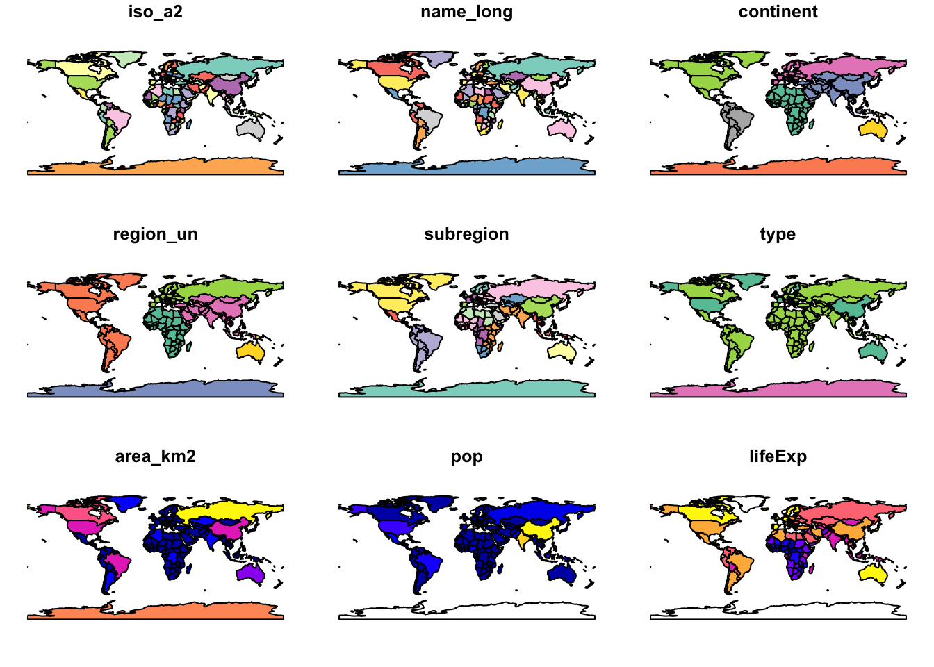
Expand here to see past versions of unnamed-chunk-29-1.png:</em></summary>
<table style="border-collapse:separate; border-spacing:5px;">
<thead>
<tr>
<th style="text-align:left;">
Version
</th>
<th style="text-align:left;">
Author
</th>
<th style="text-align:left;">
Date
</th>
</tr>
</thead>
<tbody>
<tr>
<td style="text-align:left;">
<a href="https://github.com/annakrystalli/intro-r-gis/blob/8a975bc813c1c2196785cb9a30ec849bb50c60dd/docs/figure/vector.Rmd/unnamed-chunk-29-1.png" target="_blank">8a975bc</a>
</td>
<td style="text-align:left;">
annakrystalli
</td>
<td style="text-align:left;">
2018-09-04
</td>
</tr>
</tbody>
</table>
<p></details></p>
<div class="sourceCode"><pre class="sourceCode r"><code class="sourceCode r">world_merc <span class="op">%&gt;%</span><span class="st"> </span><span class="kw">plot</span>()</code></pre></div>
<pre><code>Warning: plotting the first 9 out of 10 attributes; use max.plot = 10 to
plot all</code></pre>
<p><img src="figure/vector.Rmd/unnamed-chunk-30-1.png" width="672" style="display: block; margin: auto;" /></p>
<details> <summary><em>
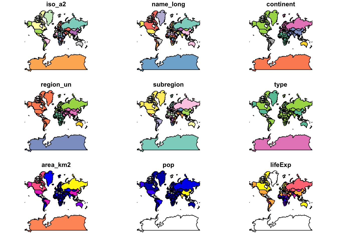
Expand here to see past versions of unnamed-chunk-30-1.png:</em></summary>
<table style="border-collapse:separate; border-spacing:5px;">
<thead>
<tr>
<th style="text-align:left;">
Version
</th>
<th style="text-align:left;">
Author
</th>
<th style="text-align:left;">
Date
</th>
</tr>
</thead>
<tbody>
<tr>
<td style="text-align:left;">
<a href="https://github.com/annakrystalli/intro-r-gis/blob/8a975bc813c1c2196785cb9a30ec849bb50c60dd/docs/figure/vector.Rmd/unnamed-chunk-30-1.png" target="_blank">8a975bc</a>
</td>
<td style="text-align:left;">
annakrystalli
</td>
<td style="text-align:left;">
2018-09-04
</td>
</tr>
</tbody>
</table>
<p></details></p>
<p>We can easily select and plot information for a single variable</p>
<div class="sourceCode"><pre class="sourceCode r"><code class="sourceCode r">world <span class="op">%&gt;%</span><span class="st"> </span><span class="kw">select</span>(lifeExp) <span class="op">%&gt;%</span><span class="st"> </span><span class="kw">plot</span>()</code></pre></div>
<p><img src="figure/vector.Rmd/unnamed-chunk-31-1.png" width="672" style="display: block; margin: auto;" /></p>
<details> <summary><em>
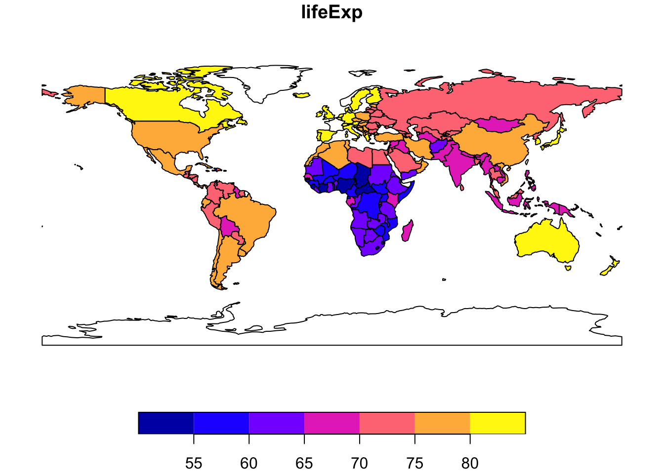
Expand here to see past versions of unnamed-chunk-31-1.png:</em></summary>
<table style="border-collapse:separate; border-spacing:5px;">
<thead>
<tr>
<th style="text-align:left;">
Version
</th>
<th style="text-align:left;">
Author
</th>
<th style="text-align:left;">
Date
</th>
</tr>
</thead>
<tbody>
<tr>
<td style="text-align:left;">
<a href="https://github.com/annakrystalli/intro-r-gis/blob/8a975bc813c1c2196785cb9a30ec849bb50c60dd/docs/figure/vector.Rmd/unnamed-chunk-31-1.png" target="_blank">8a975bc</a>
</td>
<td style="text-align:left;">
annakrystalli
</td>
<td style="text-align:left;">
2018-09-04
</td>
</tr>
</tbody>
</table>
<p></details></p>
<p>We can also extract and just plot out the geometries.</p>
<div class="sourceCode"><pre class="sourceCode r"><code class="sourceCode r">world <span class="op">%&gt;%</span><span class="st"> </span><span class="kw">st_geometry</span>() <span class="op">%&gt;%</span><span class="st"> </span><span class="kw">plot</span>()</code></pre></div>
<p><img src="figure/vector.Rmd/unnamed-chunk-32-1.png" width="672" style="display: block; margin: auto;" /></p>
<details> <summary><em>
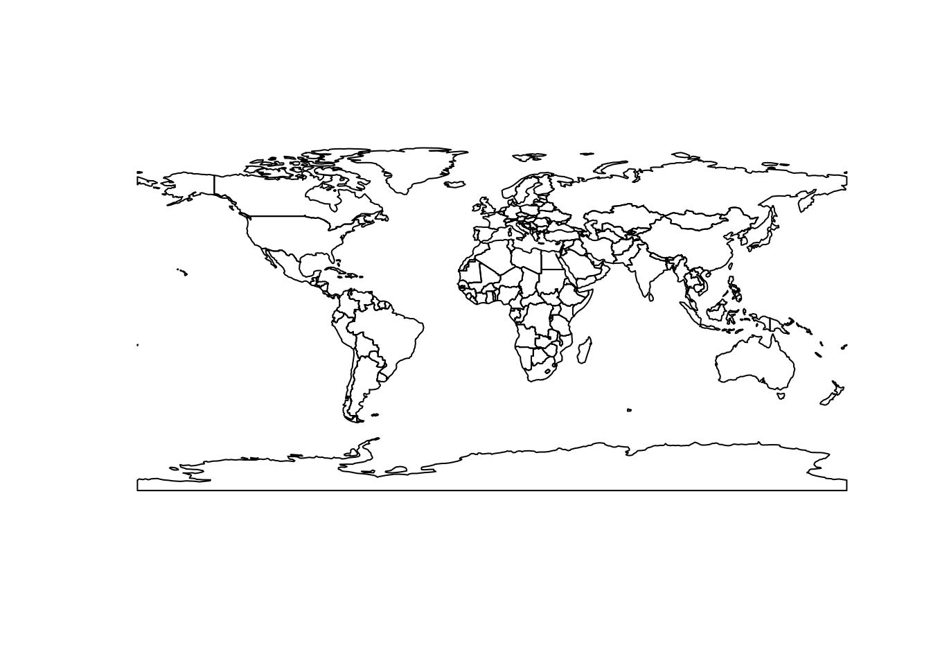
Expand here to see past versions of unnamed-chunk-32-1.png:</em></summary>
<table style="border-collapse:separate; border-spacing:5px;">
<thead>
<tr>
<th style="text-align:left;">
Version
</th>
<th style="text-align:left;">
Author
</th>
<th style="text-align:left;">
Date
</th>
</tr>
</thead>
<tbody>
<tr>
<td style="text-align:left;">
<a href="https://github.com/annakrystalli/intro-r-gis/blob/8a975bc813c1c2196785cb9a30ec849bb50c60dd/docs/figure/vector.Rmd/unnamed-chunk-32-1.png" target="_blank">8a975bc</a>
</td>
<td style="text-align:left;">
annakrystalli
</td>
<td style="text-align:left;">
2018-09-04
</td>
</tr>
</tbody>
</table>
<p></details></p>
<div id="exercises" class="section level3">
<h3>Exercises</h3>
<p><strong>2) What are the coordinates for the 10th point in the Mexico polygon?</strong></p>
<p>**3) How about in CRS <a href="https://epsg.io/4488">Mexico ITRF92 / UTM zone 15N</a></p>
<p><strong>4) Are these coordinates projected or not? Can you tell by just looking at the spatial information in the transformed <code>sf</code> object?</strong></p>
</div>
</div>
</div>
<div id="a-working-example" class="section level1">
<h1>A working example</h1>
<div id="molecular-data-on-salamanders" class="section level3">
<h3>Molecular data on salamanders</h3>
<p>The data we will work with are from the paper: <em>Tracking climate change in a dispersal‐limited species: reduced spatial and genetic connectivity in a montane salamander (2013)</em> <a href="https://doi.org/10.1111/mec.12310" class="uri">https://doi.org/10.1111/mec.12310</a></p>
<p>The researchers where interested in examining how <strong>climate and landscape features in montane regions affect population genetic structure of montane salamander</strong> <strong><em>Pseudoeurycea leprosa.</em></strong></p>
<p>To address this they used ecological niche modelling (ENM) and measured spatial connectivity and gene flow across extant populations of P. leprosa in the Trans‐Mexican Volcanic Belt (TVB).</p>
<p>To do this they had to <strong>combine their molecular data with environmental data</strong>. This is what we will try and reproduce during this workshop.</p>
<p>I’ve created a <code>.csv</code> of the published data containing the following fields, and saved it in file <code>data/csv/salamander_mol.csv</code>.</p>
<table>
<thead>
<tr class="header">
<th align="left">field</th>
<th align="left">description</th>
</tr>
</thead>
<tbody>
<tr class="odd">
<td align="left">id</td>
<td align="left">sample ID</td>
</tr>
<tr class="even">
<td align="left">locality</td>
<td align="left">sample locality</td>
</tr>
<tr class="odd">
<td align="left">n</td>
<td align="left">sample size</td>
</tr>
<tr class="even">
<td align="left">mountain_chain</td>
<td align="left">mountain chain</td>
</tr>
<tr class="odd">
<td align="left">region</td>
</tr>
<tr class="even">
<td align="left">latitude</td>
</tr>
<tr class="odd">
<td align="left">longitude</td>
</tr>
<tr class="even">
<td align="left">na</td>
<td align="left">average number of alleles</td>
</tr>
<tr class="odd">
<td align="left">he</td>
<td align="left">expected heterozygosity</td>
</tr>
<tr class="even">
<td align="left">ar</td>
<td align="left">allelic richness</td>
</tr>
<tr class="odd">
<td align="left">par</td>
<td align="left">private allelic richness</td>
</tr>
</tbody>
</table>
<p>Let’s read it in using function <code>readr::read_csv()</code>. I’m also using function <code>here::here()</code> to specify the paths in a way that is both portable and will work across different systems.</p>
<div class="sourceCode"><pre class="sourceCode r"><code class="sourceCode r">mol_df &lt;-<span class="st"> </span>readr<span class="op">::</span><span class="kw">read_csv</span>(here<span class="op">::</span><span class="kw">here</span>(<span class="st">&quot;data&quot;</span>, <span class="st">&quot;csv&quot;</span>, <span class="st">&quot;salamander_mol.csv&quot;</span>))</code></pre></div>
<p>Note also the use of <code>::</code>. This allows to call a function without loading the library (so long as the package has been installed).</p>
<p>Now, let’s have a look at the data we just loaded.</p>
<div class="sourceCode"><pre class="sourceCode r"><code class="sourceCode r">mol_df</code></pre></div>
<pre><code># A tibble: 15 x 11
      id locality       n mountain_chain   region latitude longitude    na
   &lt;int&gt; &lt;chr&gt;      &lt;int&gt; &lt;chr&gt;            &lt;chr&gt;     &lt;dbl&gt;     &lt;dbl&gt; &lt;dbl&gt;
 1     1 Nevado de…    12 Nevado de Toluca Centr…     19.2     -99.8  5.44
 2     2 Texcalyac…    29 Sierra de las C… Centr…     19.1     -99.5  8.22
 3     3 Desierto …     7 Sierra de las C… Centr…     19.3     -99.3  4.44
 4     4 Ajusco         8 Sierra de las C… Centr…     19.2     -99.3  4.22
 5     8 Calpan        34 Sierra Nevada    Centr…     19.1     -98.6 11.9 
 6     9 Atzompa       43 Sierra Nevada    Centr…     19.2     -98.6 10.3 
 7    10 Llano Gra…    15 Sierra Nevada (… Centr…     19.3     -98.7  7.78
 8    11 Rio Frio      27 Sierra Nevada (… Centr…     19.4     -98.7  7.56
 9    12 Nanacamil…    14 Sierra Nevada (… Centr…     19.5     -98.6  6.22
10    13 MalincheS      8 Malinche         Centr…     19.2     -98.0  5.00
11    14 MalincheW     17 Malinche         Centr…     19.3     -98.1  6.67
12    16 MalincheE     13 Malinche         Centr…     19.2     -98.0  6.11
13    17 Texmalaqu…     8 Pico de Orizaba  South…     18.9     -97.3  6.00
14    18 Xometla       16 Pico de Orizaba  South…     19.0     -97.2  9.11
15    19 Vigas         48 Cofre de Perote  North…     19.6     -97.1 11.8 
# ... with 3 more variables: he &lt;dbl&gt;, ar &lt;dbl&gt;, par &lt;dbl&gt;</code></pre>
</div>
<div id="converting-latlon-data-to-simple-features" class="section level2">
<h2>Converting lat/lon data to simple features</h2>
<p>Our data contains geographical coordinates in lat/lot decimal degrees. We can convert these sampling locations to <code>sf</code> geographic points using function <code>sf::st_as_sf()</code>. We can also assign a CRS, in this case we’ll assign WGS 84 which corresponds to epsg:4326.</p>
<div class="sourceCode"><pre class="sourceCode r"><code class="sourceCode r">mol_sf &lt;-<span class="st"> </span>sf<span class="op">::</span><span class="kw">st_as_sf</span>(mol_df, <span class="dt">coords =</span> <span class="kw">c</span>(<span class="st">&quot;longitude&quot;</span>, <span class="st">&quot;latitude&quot;</span>), 
                       <span class="dt">crs =</span> <span class="dv">4326</span>)</code></pre></div>
<div class="sourceCode"><pre class="sourceCode r"><code class="sourceCode r">mol_sf</code></pre></div>
<pre><code>Simple feature collection with 15 features and 9 fields
geometry type:  POINT
dimension:      XY
bbox:           xmin: -99.84806 ymin: 18.94194 xmax: -97.09056 ymax: 19.63083
epsg (SRID):    4326
proj4string:    +proj=longlat +datum=WGS84 +no_defs
# A tibble: 15 x 10
      id locality       n mountain_chain   region    na    he    ar    par
   &lt;int&gt; &lt;chr&gt;      &lt;int&gt; &lt;chr&gt;            &lt;chr&gt;  &lt;dbl&gt; &lt;dbl&gt; &lt;dbl&gt;  &lt;dbl&gt;
 1     1 Nevado de…    12 Nevado de Toluca Centr…  5.44 0.620  4.56 0.350 
 2     2 Texcalyac…    29 Sierra de las C… Centr…  8.22 0.660  5.14 0.500 
 3     3 Desierto …     7 Sierra de las C… Centr…  4.44 0.590  4.44 0.180 
 4     4 Ajusco         8 Sierra de las C… Centr…  4.22 0.490  4.05 0.0200
 5     8 Calpan        34 Sierra Nevada    Centr… 11.9  0.730  6.48 0.290 
 6     9 Atzompa       43 Sierra Nevada    Centr… 10.3  0.690  5.79 0.0800
 7    10 Llano Gra…    15 Sierra Nevada (… Centr…  7.78 0.650  5.80 0.250 
 8    11 Rio Frio      27 Sierra Nevada (… Centr…  7.56 0.570  4.77 0.130 
 9    12 Nanacamil…    14 Sierra Nevada (… Centr…  6.22 0.590  4.91 0.100 
10    13 MalincheS      8 Malinche         Centr…  5.00 0.580  4.69 0.0900
11    14 MalincheW     17 Malinche         Centr…  6.67 0.600  4.76 0.0600
12    16 MalincheE     13 Malinche         Centr…  6.11 0.560  4.73 0.210 
13    17 Texmalaqu…     8 Pico de Orizaba  South…  6.00 0.710  5.64 0.910 
14    18 Xometla       16 Pico de Orizaba  South…  9.11 0.830  6.86 0.490 
15    19 Vigas         48 Cofre de Perote  North… 11.8  0.660  5.75 1.31  
# ... with 1 more variable: geometry &lt;POINT [°]&gt;</code></pre>
</div>
</div>
<div id="plotting-sf-with-ggplot2" class="section level1">
<h1>Plotting <code>sf</code> with <code>ggplot2</code></h1>
<p>Another great new feature of <code>sf</code> is that <code>ggplot2</code> provides a dedicated function, <code>ggplot2::geom_sf()</code>, for mapping <code>sf</code>.</p>
<div id="plotting-sampling-locations" class="section level3">
<h3>Plotting sampling locations</h3>
<p>Let’s plot the sampling points we just specified.</p>
<div class="sourceCode"><pre class="sourceCode r"><code class="sourceCode r">mol_sf <span class="op">%&gt;%</span><span class="st"> </span><span class="kw">ggplot</span>() <span class="op">+</span>
<span class="st">  </span><span class="kw">geom_sf</span>() </code></pre></div>
<p><img src="figure/vector.Rmd/unnamed-chunk-38-1.png" width="672" style="display: block; margin: auto;" /></p>
<details> <summary><em>
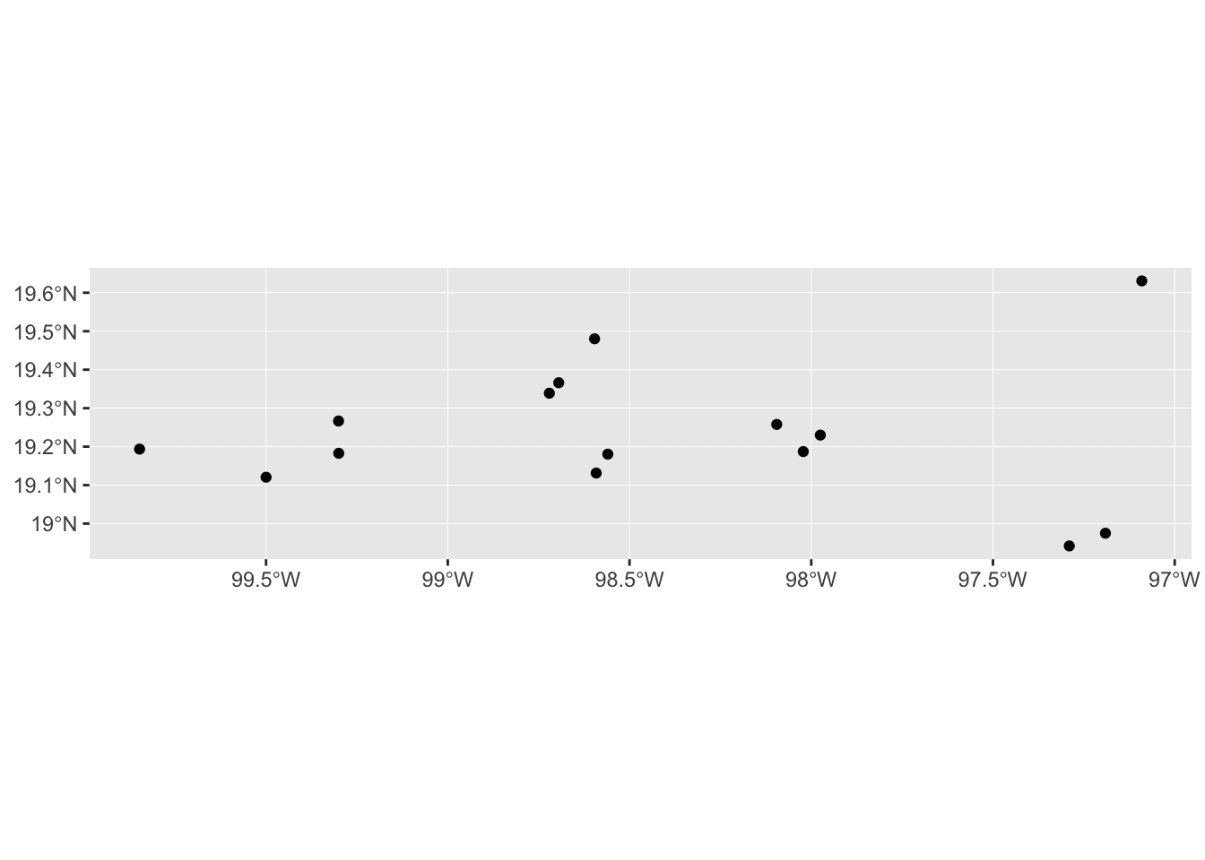
Expand here to see past versions of unnamed-chunk-38-1.png:</em></summary>
<table style="border-collapse:separate; border-spacing:5px;">
<thead>
<tr>
<th style="text-align:left;">
Version
</th>
<th style="text-align:left;">
Author
</th>
<th style="text-align:left;">
Date
</th>
</tr>
</thead>
<tbody>
<tr>
<td style="text-align:left;">
<a href="https://github.com/annakrystalli/intro-r-gis/blob/8a975bc813c1c2196785cb9a30ec849bb50c60dd/docs/figure/vector.Rmd/unnamed-chunk-38-1.png" target="_blank">8a975bc</a>
</td>
<td style="text-align:left;">
annakrystalli
</td>
<td style="text-align:left;">
2018-09-04
</td>
</tr>
</tbody>
</table>
<p></details></p>
<p>Although this doesn’t look AMAZING (yet), the coordinates are positioned correctly in space. And it also means we have the full power of <code>ggplot2</code> to add more information and customise the look of our maps.</p>
<p>For example, maybe we want to colour the points according to the number of alleles in the population.</p>
<div class="sourceCode"><pre class="sourceCode r"><code class="sourceCode r">mol_sf <span class="op">%&gt;%</span><span class="st"> </span><span class="kw">ggplot</span>() <span class="op">+</span>
<span class="st">  </span><span class="kw">geom_sf</span>(<span class="kw">aes</span>(<span class="dt">colour =</span> na)) </code></pre></div>
<p><img src="figure/vector.Rmd/unnamed-chunk-39-1.png" width="672" style="display: block; margin: auto;" /></p>
<details> <summary><em>
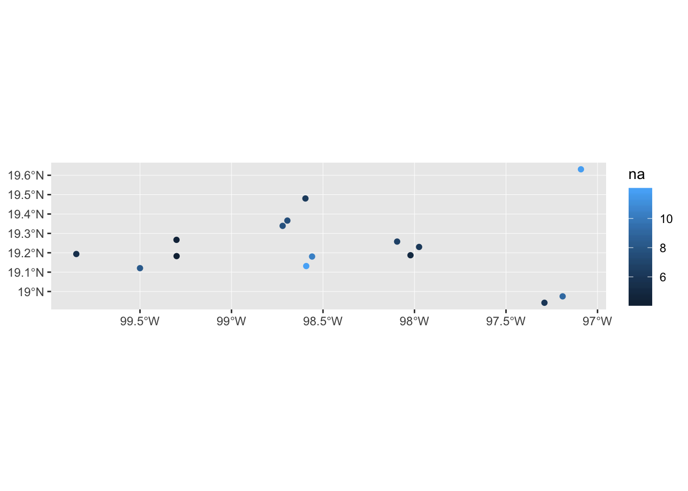
Expand here to see past versions of unnamed-chunk-39-1.png:</em></summary>
<table style="border-collapse:separate; border-spacing:5px;">
<thead>
<tr>
<th style="text-align:left;">
Version
</th>
<th style="text-align:left;">
Author
</th>
<th style="text-align:left;">
Date
</th>
</tr>
</thead>
<tbody>
<tr>
<td style="text-align:left;">
<a href="https://github.com/annakrystalli/intro-r-gis/blob/8a975bc813c1c2196785cb9a30ec849bb50c60dd/docs/figure/vector.Rmd/unnamed-chunk-39-1.png" target="_blank">8a975bc</a>
</td>
<td style="text-align:left;">
annakrystalli
</td>
<td style="text-align:left;">
2018-09-04
</td>
</tr>
</tbody>
</table>
<p></details></p>
<p>Or maybe we want to identify points by region</p>
<div class="sourceCode"><pre class="sourceCode r"><code class="sourceCode r">mol_sf <span class="op">%&gt;%</span><span class="st"> </span><span class="kw">ggplot</span>() <span class="op">+</span>
<span class="st">  </span><span class="kw">geom_sf</span>(<span class="kw">aes</span>(<span class="dt">colour =</span> region)) </code></pre></div>
<p><img src="figure/vector.Rmd/unnamed-chunk-40-1.png" width="672" style="display: block; margin: auto;" /></p>
<details> <summary><em>
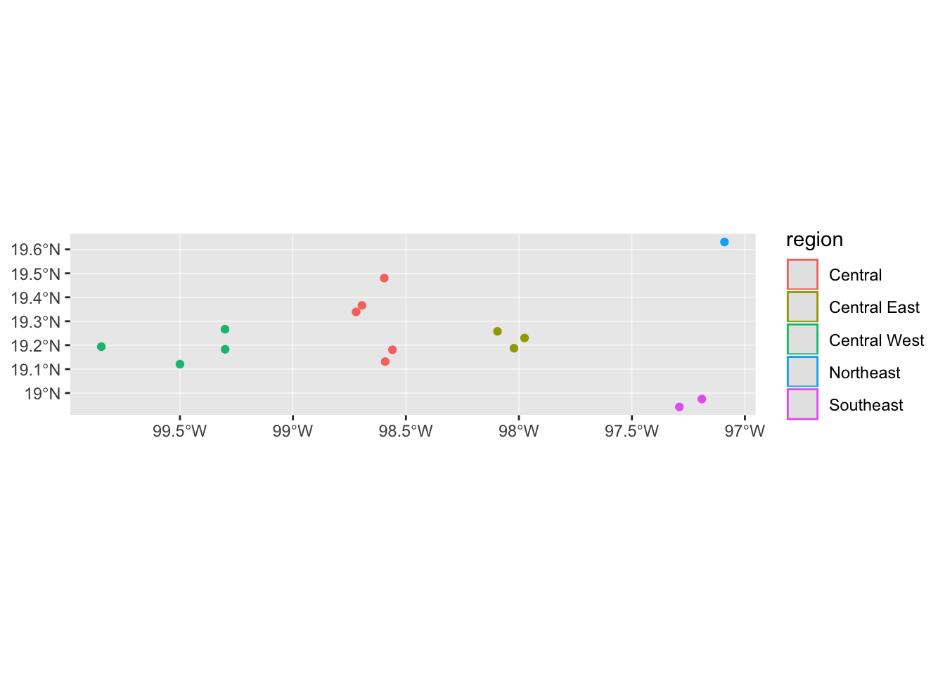
Expand here to see past versions of unnamed-chunk-40-1.png:</em></summary>
<table style="border-collapse:separate; border-spacing:5px;">
<thead>
<tr>
<th style="text-align:left;">
Version
</th>
<th style="text-align:left;">
Author
</th>
<th style="text-align:left;">
Date
</th>
</tr>
</thead>
<tbody>
<tr>
<td style="text-align:left;">
<a href="https://github.com/annakrystalli/intro-r-gis/blob/8a975bc813c1c2196785cb9a30ec849bb50c60dd/docs/figure/vector.Rmd/unnamed-chunk-40-1.png" target="_blank">8a975bc</a>
</td>
<td style="text-align:left;">
annakrystalli
</td>
<td style="text-align:left;">
2018-09-04
</td>
</tr>
</tbody>
</table>
<p></details></p>
<p>The default <code>geom_sf()</code> assumes we are plotting polygons, hence the odd legend displaying both a <code>colour</code> (outline) and a <code>fill</code> key. To get it to plot an appropriate legend for points we need to include <code>show.legend = &quot;point&quot;</code> in <code>geom_sf</code>.</p>
<div class="sourceCode"><pre class="sourceCode r"><code class="sourceCode r">mol_sf <span class="op">%&gt;%</span><span class="st"> </span><span class="kw">ggplot</span>() <span class="op">+</span>
<span class="st">  </span><span class="kw">geom_sf</span>(<span class="kw">aes</span>(<span class="dt">colour =</span> region), <span class="dt">show.legend =</span> <span class="st">&quot;point&quot;</span>) </code></pre></div>
<p><img src="figure/vector.Rmd/unnamed-chunk-41-1.png" width="672" style="display: block; margin: auto;" /></p>
<details> <summary><em>
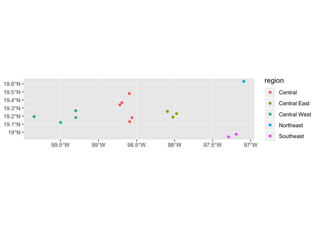
Expand here to see past versions of unnamed-chunk-41-1.png:</em></summary>
<table style="border-collapse:separate; border-spacing:5px;">
<thead>
<tr>
<th style="text-align:left;">
Version
</th>
<th style="text-align:left;">
Author
</th>
<th style="text-align:left;">
Date
</th>
</tr>
</thead>
<tbody>
<tr>
<td style="text-align:left;">
<a href="https://github.com/annakrystalli/intro-r-gis/blob/8a975bc813c1c2196785cb9a30ec849bb50c60dd/docs/figure/vector.Rmd/unnamed-chunk-41-1.png" target="_blank">8a975bc</a>
</td>
<td style="text-align:left;">
annakrystalli
</td>
<td style="text-align:left;">
2018-09-04
</td>
</tr>
</tbody>
</table>
<p></details></p>
</div>
<div id="locating-the-study-area" class="section level3">
<h3>Locating the study area</h3>
<p>We might also want to include a plot of the study area, and located in the context of the whole country.</p>
<div id="country-polygon" class="section level4">
<h4>Country polygon</h4>
<p>We can source country boundaries for Mexico from the <code>spData::world</code> <code>sf</code>.</p>
<div class="sourceCode"><pre class="sourceCode r"><code class="sourceCode r">mx &lt;-<span class="st"> </span>world <span class="op">%&gt;%</span><span class="st"> </span><span class="kw">filter</span>(name_long <span class="op">==</span><span class="st"> &quot;Mexico&quot;</span>)
mx</code></pre></div>
<pre><code>Simple feature collection with 1 feature and 10 fields
geometry type:  MULTIPOLYGON
dimension:      XY
bbox:           xmin: -117.1278 ymin: 14.53883 xmax: -86.81198 ymax: 32.72083
epsg (SRID):    4326
proj4string:    +proj=longlat +datum=WGS84 +no_defs
  iso_a2 name_long     continent region_un       subregion
1     MX    Mexico North America  Americas Central America
               type area_km2       pop lifeExp gdpPercap
1 Sovereign country  1969480 124221600  76.753   16622.6
                            geom
1 MULTIPOLYGON (((-117.1278 3...</code></pre>
</div>
<div id="study-area-bounding-box" class="section level4">
<h4>Study area bounding box</h4>
<p>Now, we also need to get the bounding box of our study area. We can use <code>sf::st_bbox()</code></p>
<div class="sourceCode"><pre class="sourceCode r"><code class="sourceCode r">study_bbox &lt;-<span class="st"> </span>mol_sf <span class="op">%&gt;%</span><span class="st"> </span>sf<span class="op">::</span><span class="kw">st_bbox</span>()
study_bbox</code></pre></div>
<pre><code>     xmin      ymin      xmax      ymax 
-99.84806  18.94194 -97.09056  19.63083 </code></pre>
<p>This just returns the coordinates specifying the boundaries of our <code>sf</code> in each dimension. We can turn this into a rectangular polygon in an <code>sfc</code> with function <code>sf::st_as_sfc</code>.</p>
<div class="sourceCode"><pre class="sourceCode r"><code class="sourceCode r">study_bbox &lt;-<span class="st"> </span>study_bbox <span class="op">%&gt;%</span><span class="st"> </span><span class="kw">st_as_sfc</span>()
study_bbox</code></pre></div>
<pre><code>Geometry set for 1 feature 
geometry type:  POLYGON
dimension:      XY
bbox:           xmin: -99.84806 ymin: 18.94194 xmax: -97.09056 ymax: 19.63083
epsg (SRID):    4326
proj4string:    +proj=longlat +datum=WGS84 +no_defs</code></pre>
<p>Let’s plot all this together:</p>
<div class="sourceCode"><pre class="sourceCode r"><code class="sourceCode r"><span class="kw">ggplot</span>() <span class="op">+</span><span class="st"> </span>
<span class="st">    </span><span class="kw">geom_sf</span>(<span class="dt">data =</span> mx, <span class="dt">colour =</span> <span class="st">&quot;black&quot;</span>, <span class="dt">fill =</span> <span class="st">&quot;lightgrey&quot;</span>) <span class="op">+</span>
<span class="st">    </span><span class="kw">geom_sf</span>(<span class="dt">data =</span> study_bbox, <span class="dt">colour =</span> <span class="st">&quot;black&quot;</span>, <span class="dt">fill =</span> <span class="st">&quot;white&quot;</span>)</code></pre></div>
<p><img src="figure/vector.Rmd/unnamed-chunk-45-1.png" width="672" style="display: block; margin: auto;" /></p>
<details> <summary><em>
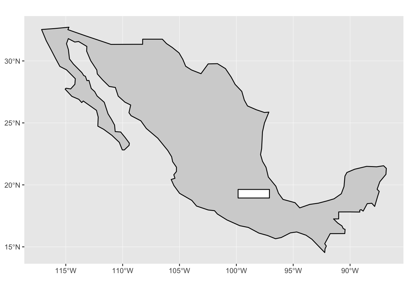
Expand here to see past versions of unnamed-chunk-45-1.png:</em></summary>
<table style="border-collapse:separate; border-spacing:5px;">
<thead>
<tr>
<th style="text-align:left;">
Version
</th>
<th style="text-align:left;">
Author
</th>
<th style="text-align:left;">
Date
</th>
</tr>
</thead>
<tbody>
<tr>
<td style="text-align:left;">
<a href="https://github.com/annakrystalli/intro-r-gis/blob/8a975bc813c1c2196785cb9a30ec849bb50c60dd/docs/figure/vector.Rmd/unnamed-chunk-45-1.png" target="_blank">8a975bc</a>
</td>
<td style="text-align:left;">
annakrystalli
</td>
<td style="text-align:left;">
2018-09-04
</td>
</tr>
</tbody>
</table>
<p></details></p>
<p>Still kinda ugly. Let’s try making the panel background a light blue.</p>
<div class="sourceCode"><pre class="sourceCode r"><code class="sourceCode r">p &lt;-<span class="st"> </span><span class="kw">ggplot</span>() <span class="op">+</span><span class="st"> </span>
<span class="st">    </span><span class="kw">theme</span>(<span class="dt">panel.background =</span> 
              <span class="kw">element_rect</span>(<span class="dt">fill =</span> <span class="st">&quot;lightblue&quot;</span>))
p</code></pre></div>
<p><img src="figure/vector.Rmd/unnamed-chunk-46-1.png" width="672" style="display: block; margin: auto;" /></p>
<details> <summary><em>Expand here to see past versions of unnamed-chunk-46-1.png:</em></summary>
<table style="border-collapse:separate; border-spacing:5px;">
<thead>
<tr>
<th style="text-align:left;">
Version
</th>
<th style="text-align:left;">
Author
</th>
<th style="text-align:left;">
Date
</th>
</tr>
</thead>
<tbody>
<tr>
<td style="text-align:left;">
<a href="https://github.com/annakrystalli/intro-r-gis/blob/8a975bc813c1c2196785cb9a30ec849bb50c60dd/docs/figure/vector.Rmd/unnamed-chunk-46-1.png" target="_blank">8a975bc</a>
</td>
<td style="text-align:left;">
annakrystalli
</td>
<td style="text-align:left;">
2018-09-04
</td>
</tr>
</tbody>
</table>
<p></details></p>
<div class="sourceCode"><pre class="sourceCode r"><code class="sourceCode r">p <span class="op">+</span><span class="st"> </span>
<span class="st">    </span><span class="kw">geom_sf</span>(<span class="dt">data =</span> mx, <span class="dt">colour =</span> <span class="st">&quot;black&quot;</span>, <span class="dt">fill =</span> <span class="st">&quot;lightgrey&quot;</span>) <span class="op">+</span>
<span class="st">    </span><span class="kw">geom_sf</span>(<span class="dt">data =</span> study_bbox, <span class="dt">colour =</span> <span class="st">&quot;black&quot;</span>, <span class="dt">fill =</span> <span class="st">&quot;white&quot;</span>) </code></pre></div>
<p><img src="figure/vector.Rmd/unnamed-chunk-47-1.png" width="672" style="display: block; margin: auto;" /></p>
<details> <summary><em>
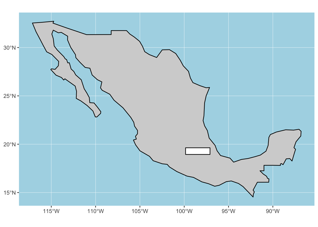
Expand here to see past versions of unnamed-chunk-47-1.png:</em></summary>
<table style="border-collapse:separate; border-spacing:5px;">
<thead>
<tr>
<th style="text-align:left;">
Version
</th>
<th style="text-align:left;">
Author
</th>
<th style="text-align:left;">
Date
</th>
</tr>
</thead>
<tbody>
<tr>
<td style="text-align:left;">
<a href="https://github.com/annakrystalli/intro-r-gis/blob/8a975bc813c1c2196785cb9a30ec849bb50c60dd/docs/figure/vector.Rmd/unnamed-chunk-47-1.png" target="_blank">8a975bc</a>
</td>
<td style="text-align:left;">
annakrystalli
</td>
<td style="text-align:left;">
2018-09-04
</td>
</tr>
</tbody>
</table>
<p></details></p>
<p>in CRS <a href="https://epsg.io/4488">Mexico ITRF92 / UTM zone 15N</a></p>
<div class="sourceCode"><pre class="sourceCode r"><code class="sourceCode r">mx_utm15 &lt;-<span class="st"> </span><span class="kw">st_transform</span>(mx, <span class="dt">crs =</span> <span class="dv">4488</span>)

p <span class="op">+</span><span class="st"> </span>
<span class="st">    </span><span class="kw">geom_sf</span>(<span class="dt">data =</span> mx_utm15, <span class="dt">colour =</span> <span class="st">&quot;black&quot;</span>, <span class="dt">fill =</span> <span class="st">&quot;lightgrey&quot;</span>) <span class="op">+</span>
<span class="st">    </span><span class="kw">geom_sf</span>(<span class="dt">data =</span> study_bbox, <span class="dt">colour =</span> <span class="st">&quot;black&quot;</span>, <span class="dt">fill =</span> <span class="st">&quot;white&quot;</span>) </code></pre></div>
<p><img src="figure/vector.Rmd/unnamed-chunk-48-1.png" width="672" style="display: block; margin: auto;" /></p>
<details> <summary><em>
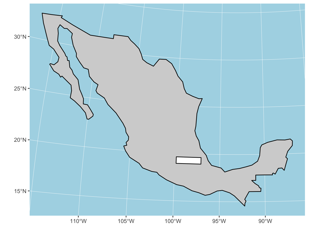
Expand here to see past versions of unnamed-chunk-48-1.png:</em></summary>
<table style="border-collapse:separate; border-spacing:5px;">
<thead>
<tr>
<th style="text-align:left;">
Version
</th>
<th style="text-align:left;">
Author
</th>
<th style="text-align:left;">
Date
</th>
</tr>
</thead>
<tbody>
<tr>
<td style="text-align:left;">
<a href="https://github.com/annakrystalli/intro-r-gis/blob/8a975bc813c1c2196785cb9a30ec849bb50c60dd/docs/figure/vector.Rmd/unnamed-chunk-48-1.png" target="_blank">8a975bc</a>
</td>
<td style="text-align:left;">
annakrystalli
</td>
<td style="text-align:left;">
2018-09-04
</td>
</tr>
</tbody>
</table>
<p></details></p>
<p>Before <code>sf_geom</code>, we could still plot geographic data. However, it took a lot more code to do so. Here’s what we’d need to code the first Mexico plot:</p>
<div class="sourceCode"><pre class="sourceCode r"><code class="sourceCode r">mx_coords &lt;-<span class="st"> </span><span class="kw">st_coordinates</span>(mx) <span class="op">%&gt;%</span><span class="st"> </span><span class="kw">as.data.frame</span>()
bbox_coords &lt;-<span class="st"> </span><span class="kw">st_coordinates</span>(study_bbox) <span class="op">%&gt;%</span><span class="st"> </span><span class="kw">as.data.frame</span>()

p <span class="op">+</span><span class="st"> </span>
<span class="st">    </span><span class="kw">geom_polygon</span>(<span class="dt">data =</span> mx_coords, <span class="kw">aes</span>(<span class="dt">x =</span> X, <span class="dt">y =</span> Y), 
                 <span class="dt">colour =</span> <span class="st">&quot;black&quot;</span>, <span class="dt">fill =</span> <span class="st">&quot;lightgrey&quot;</span>) <span class="op">+</span>
<span class="st">    </span><span class="kw">geom_polygon</span>(<span class="dt">data =</span> bbox_coords, <span class="kw">aes</span>(<span class="dt">x =</span> X, <span class="dt">y =</span> Y), 
                 <span class="dt">colour =</span> <span class="st">&quot;black&quot;</span>, <span class="dt">fill =</span> <span class="st">&quot;white&quot;</span>) <span class="op">+</span>
<span class="st">    </span><span class="kw">coord_quickmap</span>()</code></pre></div>
<p><img src="figure/vector.Rmd/unnamed-chunk-49-1.png" width="672" style="display: block; margin: auto;" /></p>
<details> <summary><em>
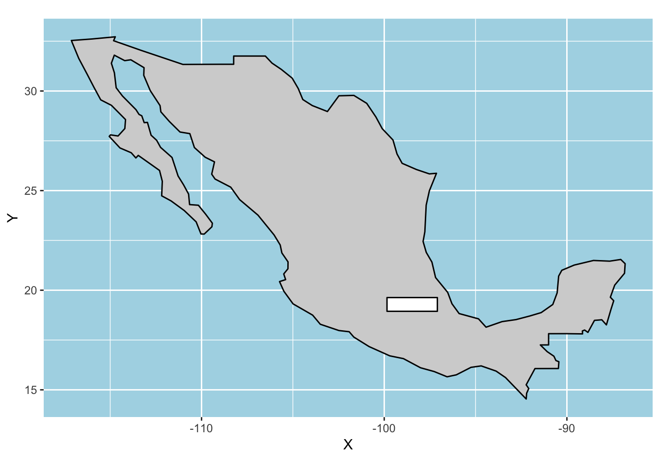
Expand here to see past versions of unnamed-chunk-49-1.png:</em></summary>
<table style="border-collapse:separate; border-spacing:5px;">
<thead>
<tr>
<th style="text-align:left;">
Version
</th>
<th style="text-align:left;">
Author
</th>
<th style="text-align:left;">
Date
</th>
</tr>
</thead>
<tbody>
<tr>
<td style="text-align:left;">
<a href="https://github.com/annakrystalli/intro-r-gis/blob/8a975bc813c1c2196785cb9a30ec849bb50c60dd/docs/figure/vector.Rmd/unnamed-chunk-49-1.png" target="_blank">8a975bc</a>
</td>
<td style="text-align:left;">
annakrystalli
</td>
<td style="text-align:left;">
2018-09-04
</td>
</tr>
</tbody>
</table>
<p></details></p>
<p>So, firstly we needed our data to be in a data.frame with a column for each of the x and y coordinates. Then we would need to use the appropriate <code>geom_*()</code> function according to the shape we are trying to plot (in this case <code>geom_polygon()</code>. If we wanted to plot points we would use <code>geom_point()</code>). We need to specify the columns that contain the x &amp; y coordinates and finally, we also need to include <code>coord_quickmap()</code> which projects our points geographically.</p>
<p>That’s a lot more work that’s handled automatically by <code>geom_sf</code>. Most importantly, when overlaying shapes, <strong><code>ggplot2</code> has no idea about projections!</strong></p>
<p>If you remember, in our previous UTM 15 example, we only transformed the first layer we plotted (ie <code>mx</code> to <code>mx_utm15</code>). When <code>study_bbox</code> was plotted subsequently, it’s CRS was automatically transformed to that of the <code>mx_utm15</code>.</p>
<p>If we try the same with <code>geom_polygon</code>, the coordinates for the two layers are now in completely different CRSs and the study bounding box does not even show up on the map!</p>
<div class="sourceCode"><pre class="sourceCode r"><code class="sourceCode r">mx_utm15_coords &lt;-<span class="st"> </span><span class="kw">st_coordinates</span>(mx_utm15) <span class="op">%&gt;%</span><span class="st"> </span><span class="kw">as.data.frame</span>()
bbox_coords &lt;-<span class="st"> </span><span class="kw">st_coordinates</span>(study_bbox) <span class="op">%&gt;%</span><span class="st"> </span><span class="kw">as.data.frame</span>()

p <span class="op">+</span><span class="st"> </span>
<span class="st">    </span><span class="kw">geom_polygon</span>(<span class="dt">data =</span> mx_utm15_coords, 
                 <span class="kw">aes</span>(<span class="dt">x =</span> X, <span class="dt">y =</span> Y), <span class="dt">colour =</span> <span class="st">&quot;black&quot;</span>, <span class="dt">fill =</span> <span class="st">&quot;lightgrey&quot;</span>) <span class="op">+</span>
<span class="st">    </span><span class="kw">geom_polygon</span>(<span class="dt">data =</span> bbox_coords, 
                 <span class="kw">aes</span>(<span class="dt">x =</span> X, <span class="dt">y =</span> Y), <span class="dt">colour =</span> <span class="st">&quot;black&quot;</span>, <span class="dt">fill =</span> <span class="st">&quot;white&quot;</span>) <span class="op">+</span>
<span class="st">    </span><span class="kw">coord_quickmap</span>()</code></pre></div>
<p><img src="figure/vector.Rmd/unnamed-chunk-50-1.png" width="672" style="display: block; margin: auto;" /></p>
<details> <summary><em>
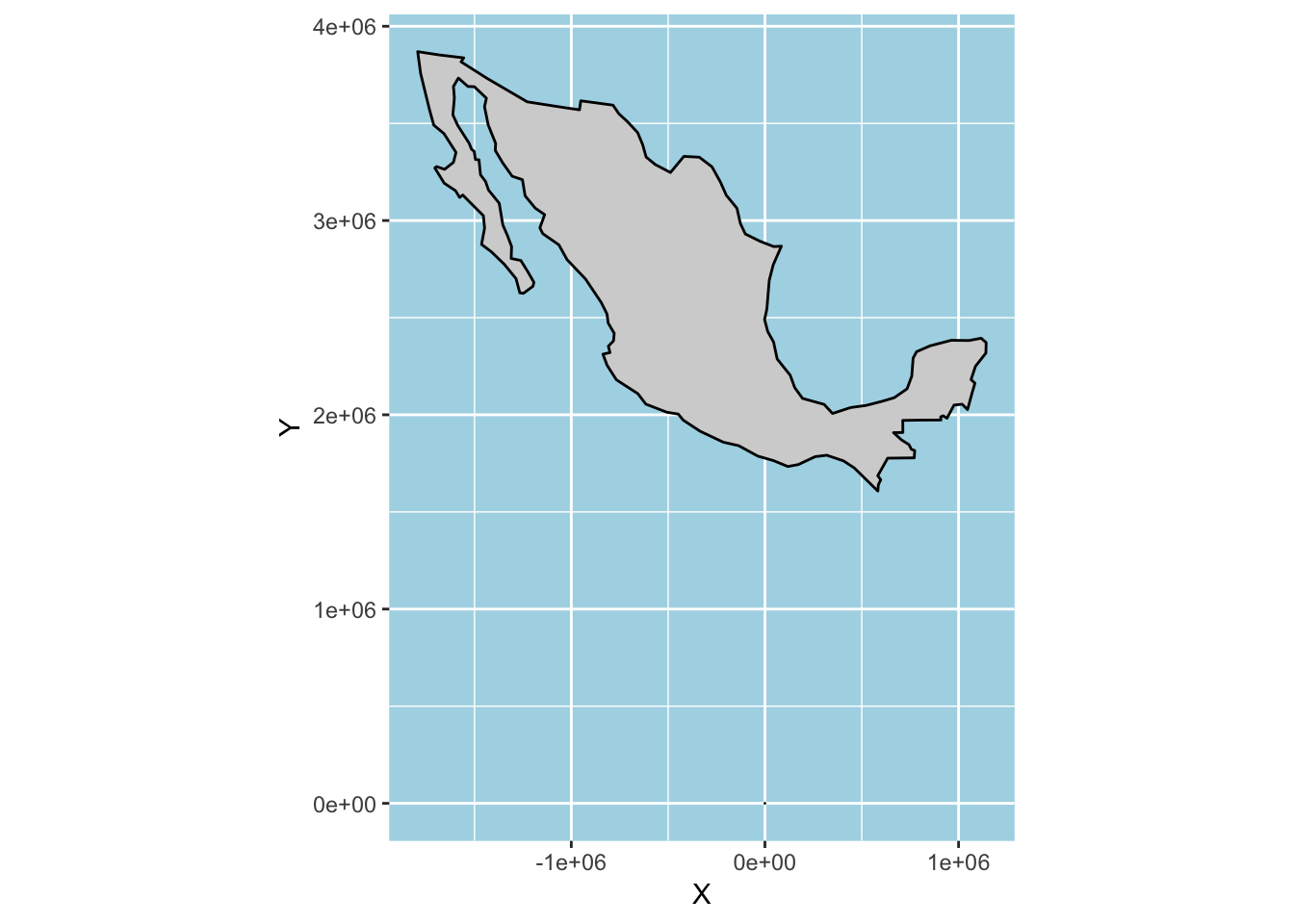
Expand here to see past versions of unnamed-chunk-50-1.png:</em></summary>
<table style="border-collapse:separate; border-spacing:5px;">
<thead>
<tr>
<th style="text-align:left;">
Version
</th>
<th style="text-align:left;">
Author
</th>
<th style="text-align:left;">
Date
</th>
</tr>
</thead>
<tbody>
<tr>
<td style="text-align:left;">
<a href="https://github.com/annakrystalli/intro-r-gis/blob/8a975bc813c1c2196785cb9a30ec849bb50c60dd/docs/figure/vector.Rmd/unnamed-chunk-50-1.png" target="_blank">8a975bc</a>
</td>
<td style="text-align:left;">
annakrystalli
</td>
<td style="text-align:left;">
2018-09-04
</td>
</tr>
</tbody>
</table>
<p></details></p>
<p>Also, the axis units… yuk!</p>
</div>
</div>
</div>
<div id="saving-sf-objects" class="section level1">
<h1>Saving <code>sf</code> objects</h1>
<p>Package <code>sf</code> provides a variety of drivers allowing us to write geospatial vector data to a number of file formats:</p>
<div class="sourceCode"><pre class="sourceCode r"><code class="sourceCode r">sf<span class="op">::</span><span class="kw">st_drivers</span>() <span class="op">%&gt;%</span><span class="st"> </span>DT<span class="op">::</span><span class="kw">datatable</span>()</code></pre></div>
<div id="htmlwidget-33beb40a5948c9b22760" style="width:100%;height:auto;" class="datatables html-widget"></div>
<script type="application/json" data-for="htmlwidget-33beb40a5948c9b22760">{"x":{"filter":"none","data":[["PCIDSK","netCDF","PDF","ESRI Shapefile","MapInfo File","UK .NTF","OGR_SDTS","S57","DGN","OGR_VRT","REC","Memory","BNA","CSV","GML","GPX","KML","GeoJSON","OGR_GMT","GPKG","SQLite","WAsP","OpenFileGDB","XPlane","DXF","Geoconcept","GeoRSS","GPSTrackMaker","VFK","PGDUMP","OSM","GPSBabel","SUA","OpenAir","OGR_PDS","WFS","HTF","AeronavFAA","EDIGEO","GFT","SVG","CouchDB","Cloudant","Idrisi","ARCGEN","SEGUKOOA","SEGY","ODS","XLSX","ElasticSearch","Carto","AmigoCloud","SXF","Selafin","JML","PLSCENES","CSW","VDV","TIGER","AVCBin","AVCE00","HTTP"],["PCIDSK","netCDF","PDF","ESRI Shapefile","MapInfo File","UK .NTF","OGR_SDTS","S57","DGN","OGR_VRT","REC","Memory","BNA","CSV","GML","GPX","KML","GeoJSON","OGR_GMT","GPKG","SQLite","WAsP","OpenFileGDB","XPlane","DXF","Geoconcept","GeoRSS","GPSTrackMaker","VFK","PGDUMP","OSM","GPSBabel","SUA","OpenAir","OGR_PDS","WFS","HTF","AeronavFAA","EDIGEO","GFT","SVG","CouchDB","Cloudant","Idrisi","ARCGEN","SEGUKOOA","SEGY","ODS","XLSX","ElasticSearch","Carto","AmigoCloud","SXF","Selafin","JML","PLSCENES","CSW","VDV","TIGER","AVCBin","AVCE00","HTTP"],["PCIDSK Database File","Network Common Data Format","Geospatial PDF","ESRI Shapefile","MapInfo File","UK .NTF","SDTS","IHO S-57 (ENC)","Microstation DGN","VRT - Virtual Datasource","EPIInfo .REC ","Memory","Atlas BNA","Comma Separated Value (.csv)","Geography Markup Language (GML)","GPX","Keyhole Markup Language (KML)","GeoJSON","GMT ASCII Vectors (.gmt)","GeoPackage","SQLite / Spatialite","WAsP .map format","ESRI FileGDB","X-Plane/Flightgear aeronautical data","AutoCAD DXF","Geoconcept","GeoRSS","GPSTrackMaker","Czech Cadastral Exchange Data Format","PostgreSQL SQL dump","OpenStreetMap XML and PBF","GPSBabel","Tim Newport-Peace's Special Use Airspace Format","OpenAir","Planetary Data Systems TABLE","OGC WFS (Web Feature Service)","Hydrographic Transfer Vector","Aeronav FAA","French EDIGEO exchange format","Google Fusion Tables","Scalable Vector Graphics","CouchDB / GeoCouch","Cloudant / CouchDB","Idrisi Vector (.vct)","Arc/Info Generate","SEG-P1 / UKOOA P1/90","SEG-Y","Open Document/ LibreOffice / OpenOffice Spreadsheet ","MS Office Open XML spreadsheet","Elastic Search","Carto","AmigoCloud","Storage and eXchange Format","Selafin","OpenJUMP JML","Planet Labs Scenes API","OGC CSW (Catalog  Service for the Web)","VDV-451/VDV-452/INTREST Data Format","U.S. Census TIGER/Line","Arc/Info Binary Coverage","Arc/Info E00 (ASCII) Coverage","HTTP Fetching Wrapper"],[true,true,true,true,true,false,false,true,true,false,false,true,true,true,true,true,true,true,true,true,true,true,false,false,true,true,true,true,false,true,false,true,false,false,false,false,false,false,false,true,false,true,true,false,false,false,false,true,true,true,true,true,false,true,true,false,false,true,true,false,false,false],[false,true,true,false,false,false,false,false,false,false,false,false,false,false,false,false,false,false,false,true,false,false,false,false,false,false,false,false,false,false,false,false,false,false,false,false,false,false,false,false,false,false,false,false,false,false,false,false,false,false,false,false,false,false,false,false,false,false,false,false,false,false],[true,true,true,false,false,false,false,false,false,false,false,false,false,false,false,false,false,false,false,true,false,false,false,false,false,false,false,false,false,false,false,false,false,false,false,false,false,false,false,false,false,false,false,false,false,false,false,false,false,false,false,false,false,false,false,true,false,false,false,false,false,true],[true,true,true,true,true,true,true,true,true,true,true,true,true,true,true,true,true,true,true,true,true,true,true,true,true,true,true,true,true,true,true,true,true,true,true,true,true,true,true,true,true,true,true,true,true,true,true,true,true,true,true,true,true,true,true,true,true,true,true,true,true,true],[true,false,false,true,true,false,false,true,false,true,false,false,true,true,true,true,true,true,false,true,true,true,true,true,true,false,true,true,false,true,true,false,true,true,true,true,true,true,true,false,true,false,false,true,true,true,true,true,true,false,false,false,false,true,true,false,false,true,true,false,false,false]],"container":"<table class=\"display\">\n  <thead>\n    <tr>\n      <th> <\/th>\n      <th>name<\/th>\n      <th>long_name<\/th>\n      <th>write<\/th>\n      <th>copy<\/th>\n      <th>is_raster<\/th>\n      <th>is_vector<\/th>\n      <th>vsi<\/th>\n    <\/tr>\n  <\/thead>\n<\/table>","options":{"order":[],"autoWidth":false,"orderClasses":false,"columnDefs":[{"orderable":false,"targets":0}]}},"evals":[],"jsHooks":[]}</script>
<p>Let’s first create a new folder to save our <code>sf</code>.</p>
<div class="sourceCode"><pre class="sourceCode r"><code class="sourceCode r"><span class="kw">dir.create</span>(here<span class="op">::</span><span class="kw">here</span>(<span class="st">&quot;data&quot;</span>, <span class="st">&quot;sf&quot;</span>))</code></pre></div>
<div id="shapefiles-.shp" class="section level2">
<h2>shapefiles (<code>.shp</code>)</h2>
<p>Let’s now save our file in the most popular geospatial vector data format, the <a href="https://en.wikipedia.org/wiki/Shapefile">shapefile(<code>.shp</code>)</a>. It is developed and regulated by Esri as a (mostly) open specification for data interoperability among Esri and other GIS software products.</p>
<div class="sourceCode"><pre class="sourceCode r"><code class="sourceCode r"><span class="kw">write_sf</span>(mol_sf, here<span class="op">::</span><span class="kw">here</span>(<span class="st">&quot;data&quot;</span>, <span class="st">&quot;sf&quot;</span>, <span class="st">&quot;salamander.shp&quot;</span>))</code></pre></div>
<pre><code>Warning in abbreviate_shapefile_names(obj): Field names abbreviated for
ESRI Shapefile driver</code></pre>
<pre><code>Warning in CPL_write_ogr(obj, dsn, layer, driver, as.character(dataset_options), : GDAL Message 1: One or several characters couldn&#39;t be converted correctly from UTF-8 to ISO-8859-1.
This warning will not be emitted anymore.</code></pre>
<p>Hmmmmm, that’s a bit of a worrying warning…but let’s have a quick look at what we just wrote out anyways.</p>
<p>If you look in the <code>sf/</code> folder, you will see that <strong>four files have been created</strong> for each <code>sf</code> we wrote. Here’s what each file contains:</p>
<ul>
<li><p><strong><code>.shp</code>:</strong> This file contains the geometry of each feature.</p></li>
<li><p><strong><code>.dbf</code>:</strong> This is a dBase file which contains the attribute data for all of the features in the dataset. The dBase file is very similar to a sheet in a spreadsheet and can even be opened in Excel.</p></li>
<li><p><strong><code>.shx</code>:</strong> The .shx is the spatial index, it allows GIS systems to find features within the <code>.shp</code> file more quickly.</p></li>
<li><p><strong><code>.prj</code>:</strong> The .prj is the projection file. It contains information about the “projection” and “coordinate system” of the data.</p></li>
</ul>
<p>All of them are required to fully recreate our <code>sf</code> but when to read the data in, you <strong>only specify the path to the <code>.shp</code> file</strong></p>
<p>Now, as noted, I really didn’t like the look of that previous warning, so let’s read in the file and have a look at it.</p>
<div class="sourceCode"><pre class="sourceCode r"><code class="sourceCode r"><span class="kw">read_sf</span>(here<span class="op">::</span><span class="kw">here</span>(<span class="st">&quot;data&quot;</span>, <span class="st">&quot;sf&quot;</span>, <span class="st">&quot;salamander.shp&quot;</span>))</code></pre></div>
<pre><code>Simple feature collection with 15 features and 9 fields
geometry type:  POINT
dimension:      XY
bbox:           xmin: -99.84806 ymin: 18.94194 xmax: -97.09056 ymax: 19.63083
epsg (SRID):    4326
proj4string:    +proj=longlat +datum=WGS84 +no_defs
# A tibble: 15 x 10
      id localty         n mntn_ch        region     na    he    ar    par
   &lt;int&gt; &lt;chr&gt;       &lt;int&gt; &lt;chr&gt;          &lt;chr&gt;   &lt;dbl&gt; &lt;dbl&gt; &lt;dbl&gt;  &lt;dbl&gt;
 1     1 Nevado de …    12 Nevado de Tol… Centra…  5.44 0.620  4.56 0.350 
 2     2 Texcalyacac    29 Sierra de las… Centra…  8.22 0.660  5.14 0.500 
 3     3 Desierto d…     7 Sierra de las… Centra…  4.44 0.590  4.44 0.180 
 4     4 Ajusco          8 Sierra de las… Centra…  4.22 0.490  4.05 0.0200
 5     8 Calpan         34 Sierra Nevada  Central 11.9  0.730  6.48 0.290 
 6     9 Atzompa        43 Sierra Nevada  Central 10.3  0.690  5.79 0.0800
 7    10 Llano Gran…    15 Sierra Nevada… Central  7.78 0.650  5.80 0.250 
 8    11 Rio Frio       27 Sierra Nevada… Central  7.56 0.570  4.77 0.130 
 9    12 Nanacamilpa    14 Sierra Nevada… Central  6.22 0.590  4.91 0.100 
10    13 MalincheS       8 Malinche       Centra…  5.00 0.580  4.69 0.0900
11    14 MalincheW      17 Malinche       Centra…  6.67 0.600  4.76 0.0600
12    16 MalincheE      13 Malinche       Centra…  6.11 0.560  4.73 0.210 
13    17 Texmalaqui…     8 Pico de Oriza… Southe…  6.00 0.710  5.64 0.910 
14    18 Xometla        16 Pico de Oriza… Southe…  9.11 0.830  6.86 0.490 
15    19 Vigas          48 Cofre de Pero… Northe… 11.8  0.660  5.75 1.31  
# ... with 1 more variable: geometry &lt;POINT [°]&gt;</code></pre>
<p>Gah!! What’s happened to the column names?! This is in fact a well known problem with the shapefile format which cannot handle field (column) names longer than 7 characters. When your column names are longer than that, <code>write_sf()</code> quietly runs <code>base::abbreviate()</code> on them before writing the files out. This does not sit well with me in terms of good data provenance tracking and reproducibility. So let’s try a different format instead.</p>
</div>
<div id="geojson-.geojson" class="section level2">
<h2>GeoJSON (<code>.geojson</code>)</h2>
<p><a href="https://en.wikipedia.org/wiki/GeoJSON">GeoJSON</a> is an open standard format designed for representing simple geographical features, along with their non-spatial attributes. It differs from other GIS standards in that it was written and is maintained not by a formal standards organization, but by an Internet working group of developers. As such, it does not play well with Esri products like ArcGIS (although they can be converted to formats that will). However, if you are not planning to use your data with Esri products, this format is fine.</p>
<div class="sourceCode"><pre class="sourceCode r"><code class="sourceCode r"><span class="kw">write_sf</span>(mol_sf, here<span class="op">::</span><span class="kw">here</span>(<span class="st">&quot;data&quot;</span>, <span class="st">&quot;sf&quot;</span>, <span class="st">&quot;salamander.geojson&quot;</span>))</code></pre></div>
<p>Let’s read it back in and check it:</p>
<div class="sourceCode"><pre class="sourceCode r"><code class="sourceCode r"><span class="kw">read_sf</span>(here<span class="op">::</span><span class="kw">here</span>(<span class="st">&quot;data&quot;</span>, <span class="st">&quot;sf&quot;</span>, <span class="st">&quot;salamander.geojson&quot;</span>))</code></pre></div>
<pre><code>Simple feature collection with 15 features and 9 fields
geometry type:  POINT
dimension:      XY
bbox:           xmin: -99.84806 ymin: 18.94194 xmax: -97.09056 ymax: 19.63083
epsg (SRID):    4326
proj4string:    +proj=longlat +datum=WGS84 +no_defs
# A tibble: 15 x 10
      id locality       n mountain_chain   region    na    he    ar    par
   &lt;int&gt; &lt;chr&gt;      &lt;int&gt; &lt;chr&gt;            &lt;chr&gt;  &lt;dbl&gt; &lt;dbl&gt; &lt;dbl&gt;  &lt;dbl&gt;
 1     1 Nevado de…    12 Nevado de Toluca Centr…  5.44 0.620  4.56 0.350 
 2     2 Texcalyac…    29 Sierra de las C… Centr…  8.22 0.660  5.14 0.500 
 3     3 Desierto …     7 Sierra de las C… Centr…  4.44 0.590  4.44 0.180 
 4     4 Ajusco         8 Sierra de las C… Centr…  4.22 0.490  4.05 0.0200
 5     8 Calpan        34 Sierra Nevada    Centr… 11.9  0.730  6.48 0.290 
 6     9 Atzompa       43 Sierra Nevada    Centr… 10.3  0.690  5.79 0.0800
 7    10 Llano Gra…    15 Sierra Nevada (… Centr…  7.78 0.650  5.80 0.250 
 8    11 Rio Frio      27 Sierra Nevada (… Centr…  7.56 0.570  4.77 0.130 
 9    12 Nanacamil…    14 Sierra Nevada (… Centr…  6.22 0.590  4.91 0.100 
10    13 MalincheS      8 Malinche         Centr…  5.00 0.580  4.69 0.0900
11    14 MalincheW     17 Malinche         Centr…  6.67 0.600  4.76 0.0600
12    16 MalincheE     13 Malinche         Centr…  6.11 0.560  4.73 0.210 
13    17 Texmalaqu…     8 Pico de Orizaba  South…  6.00 0.710  5.64 0.910 
14    18 Xometla       16 Pico de Orizaba  South…  9.11 0.830  6.86 0.490 
15    19 Vigas         48 Cofre de Perote  North… 11.8  0.660  5.75 1.31  
# ... with 1 more variable: geometry &lt;POINT [°]&gt;</code></pre>
<p>Beautiful! The file is accurately reproduced with all column names intact 💪, so no need to go updating your data README or attribute metadata table.</p>
</div>
<div id="session-information" class="section level2">
<h2>Session information</h2>
<div class="sourceCode"><pre class="sourceCode r"><code class="sourceCode r"><span class="kw">sessionInfo</span>()</code></pre></div>
<pre><code>R version 3.4.4 (2018-03-15)
Platform: x86_64-apple-darwin15.6.0 (64-bit)
Running under: macOS High Sierra 10.13.3

Matrix products: default
BLAS: /Library/Frameworks/R.framework/Versions/3.4/Resources/lib/libRblas.0.dylib
LAPACK: /Library/Frameworks/R.framework/Versions/3.4/Resources/lib/libRlapack.dylib

locale:
[1] en_GB.UTF-8/en_GB.UTF-8/en_GB.UTF-8/C/en_GB.UTF-8/en_GB.UTF-8

attached base packages:
[1] stats     graphics  grDevices utils     datasets  methods   base     

other attached packages:
[1] bindrcpp_0.2.2 spData_0.2.9.3 dplyr_0.7.6    ggplot2_3.0.0 
[5] sf_0.6-3      

loaded via a namespace (and not attached):
 [1] tidyselect_0.2.4  purrr_0.2.5       colorspace_1.3-2 
 [4] htmltools_0.3.6   emo_0.0.0.9000    yaml_2.1.19      
 [7] utf8_1.1.3        rlang_0.2.1       later_0.7.3      
[10] R.oo_1.21.0       e1071_1.6-8       pillar_1.2.1     
[13] glue_1.2.0.9000   withr_2.1.2       DBI_1.0.0        
[16] R.utils_2.6.0     bindr_0.1.1       plyr_1.8.4       
[19] stringr_1.3.1     munsell_0.5.0     gtable_0.2.0     
[22] workflowr_1.0.1   R.methodsS3_1.7.1 htmlwidgets_1.2  
[25] evaluate_0.11     labeling_0.3      knitr_1.20       
[28] httpuv_1.4.4.2    crosstalk_1.0.0   class_7.3-14     
[31] highr_0.6         Rcpp_0.12.18      xtable_1.8-2     
[34] readr_1.1.1       promises_1.0.1    scales_1.0.0     
[37] backports_1.1.2   classInt_0.1-24   DT_0.4           
[40] jsonlite_1.5      mime_0.5          hms_0.4.2        
[43] digest_0.6.15     stringi_1.2.4     shiny_1.1.0      
[46] grid_3.4.4        rprojroot_1.3-2   here_0.1         
[49] cli_1.0.0         tools_3.4.4       magrittr_1.5     
[52] lazyeval_0.2.1    tibble_1.4.2      crayon_1.3.4     
[55] whisker_0.3-2     pkgconfig_2.0.2   lubridate_1.7.4  
[58] assertthat_0.2.0  rmarkdown_1.10    R6_2.2.2         
[61] units_0.6-0       git2r_0.21.0      compiler_3.4.4   </code></pre>
</div>
</div>

<!-- Adjust MathJax settings so that all math formulae are shown using
TeX fonts only; see
http://docs.mathjax.org/en/latest/configuration.html.  This will make
the presentation more consistent at the cost of the webpage sometimes
taking slightly longer to load. Note that this only works because the
footer is added to webpages before the MathJax javascript. -->
<script type="text/x-mathjax-config">
  MathJax.Hub.Config({
    "HTML-CSS": { availableFonts: ["TeX"] }
  });
</script>

<hr>
<p>
  This reproducible <a href="http://rmarkdown.rstudio.com">R Markdown</a>
  analysis was created with
  <a href="https://github.com/jdblischak/workflowr">workflowr</a> 1.0.1
</p>
<hr>


</div>
</div>

</div>

<script>

// add bootstrap table styles to pandoc tables
function bootstrapStylePandocTables() {
  $('tr.header').parent('thead').parent('table').addClass('table table-condensed');
}
$(document).ready(function () {
  bootstrapStylePandocTables();
});


</script>

<!-- dynamically load mathjax for compatibility with self-contained -->
<script>
  (function () {
    var script = document.createElement("script");
    script.type = "text/javascript";
    script.src  = "https://mathjax.rstudio.com/latest/MathJax.js?config=TeX-AMS-MML_HTMLorMML";
    document.getElementsByTagName("head")[0].appendChild(script);
  })();
</script>

</body>
</html>