smashrobust
Dongyue Xie
2018-10-02
Last updated: 2018-10-02
workflowr checks: (Click a bullet for more information)-
✔ R Markdown file: up-to-date
Great! Since the R Markdown file has been committed to the Git repository, you know the exact version of the code that produced these results.
-
✔ Environment: empty
Great job! The global environment was empty. Objects defined in the global environment can affect the analysis in your R Markdown file in unknown ways. For reproduciblity it’s best to always run the code in an empty environment.
-
✔ Seed:
set.seed(20180501)The command
set.seed(20180501)was run prior to running the code in the R Markdown file. Setting a seed ensures that any results that rely on randomness, e.g. subsampling or permutations, are reproducible. -
✔ Session information: recorded
Great job! Recording the operating system, R version, and package versions is critical for reproducibility.
-
Great! You are using Git for version control. Tracking code development and connecting the code version to the results is critical for reproducibility. The version displayed above was the version of the Git repository at the time these results were generated.✔ Repository version: 4f4e8fc
Note that you need to be careful to ensure that all relevant files for the analysis have been committed to Git prior to generating the results (you can usewflow_publishorwflow_git_commit). workflowr only checks the R Markdown file, but you know if there are other scripts or data files that it depends on. Below is the status of the Git repository when the results were generated:
Note that any generated files, e.g. HTML, png, CSS, etc., are not included in this status report because it is ok for generated content to have uncommitted changes.Ignored files: Ignored: .DS_Store Ignored: .Rhistory Untracked files: Untracked: analysis/literature.Rmd Unstaged changes: Modified: analysis/index.Rmd Modified: analysis/sigma.Rmd
Expand here to see past versions:
We see that smash.gaus still gives similar mean estimations given inaccurate variance(to ones given accurate variance) in previous section. We now try some more examples on this.
spike mean
library(smashr)
n = 2^9
t = 1:n/n
spike.f = function(x) (0.75 * exp(-500 * (x - 0.23)^2) +
            1.5  * exp(-2000 * (x - 0.33)^2) +
        3    * exp(-8000 * (x - 0.47)^2) +
            2.25 * exp(-16000 * (x - 0.69)^2) +
        0.5  * exp(-32000 * (x - 0.83)^2))
mu.s = spike.f(t)

# Scale the signal to be between 0.2 and 0.8.
mu.t = (1 + mu.s)/5
plot(mu.t, type = "l",main='main function')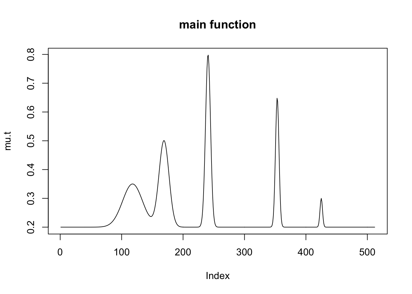
Expand here to see past versions of unnamed-chunk-1-1.png:
| Version | Author | Date |
|---|---|---|
| e7afb4d | Dongyue Xie | 2018-10-02 |
# Create the baseline variance function. (The function V2 from Cai &
# Wang 2008 is used here.)
var.fn = (1e-04 + 4 * (exp(-550 * (t - 0.2)^2) +
  exp(-200 * (t - 0.5)^2) + exp(-950 * (t - 0.8)^2)))/1.35+1
#plot(var.fn, type = "l")

# Set the signal-to-noise ratio.
rsnr = sqrt(3)
sigma.t = sqrt(var.fn)/mean(sqrt(var.fn)) * sd(mu.t)/rsnr^2
set.seed(12345)
y=mu.t+rnorm(n,0,sigma.t)
plot(y,col='grey80',main='n=512,SNR=3')
lines(smash.gaus(y))
lines(smash.gaus(y,mean(sigma.t)),col=2)
lines(smash.gaus(y,sigma.t),col=3)
lines(mu.t,col='grey80')
legend('topleft',c('smashu','smash.mean.sigma','smash.true.sigma','true mean'),col=c(1,2,3,'grey80'),lty=c(1,1,1,1))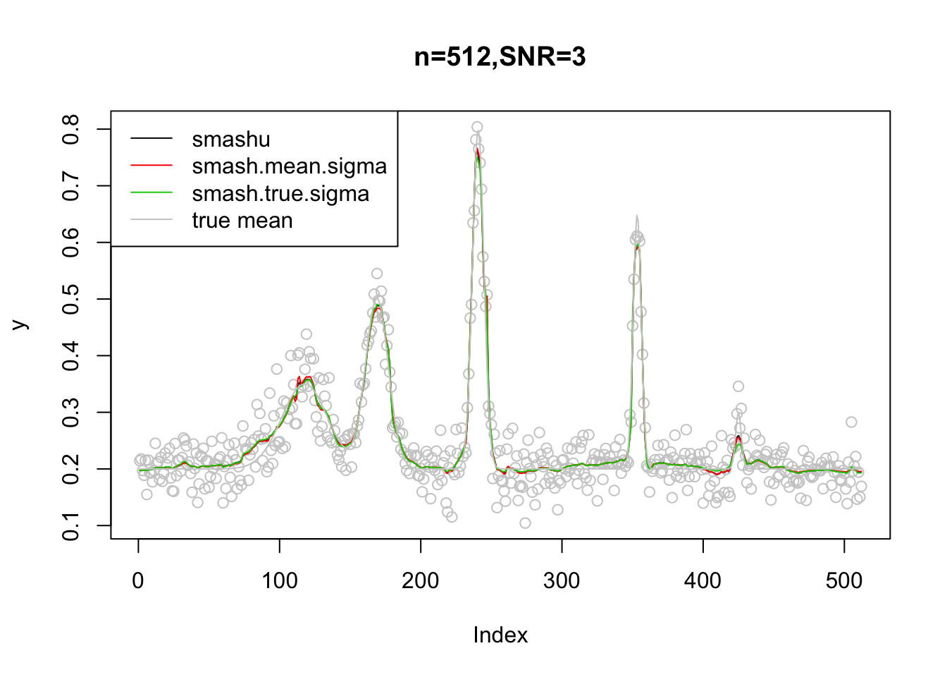
Expand here to see past versions of unnamed-chunk-2-1.png:
| Version | Author | Date |
|---|---|---|
| aacfc46 | Dongyue Xie | 2018-10-02 |
plot(sqrt(smash.gaus(y,joint=T)$var.res),type='l',ylim=c(0.02,0.05),main='sigma')
lines(rep(mean(sigma.t),n),col=2)
lines(sigma.t,col=3)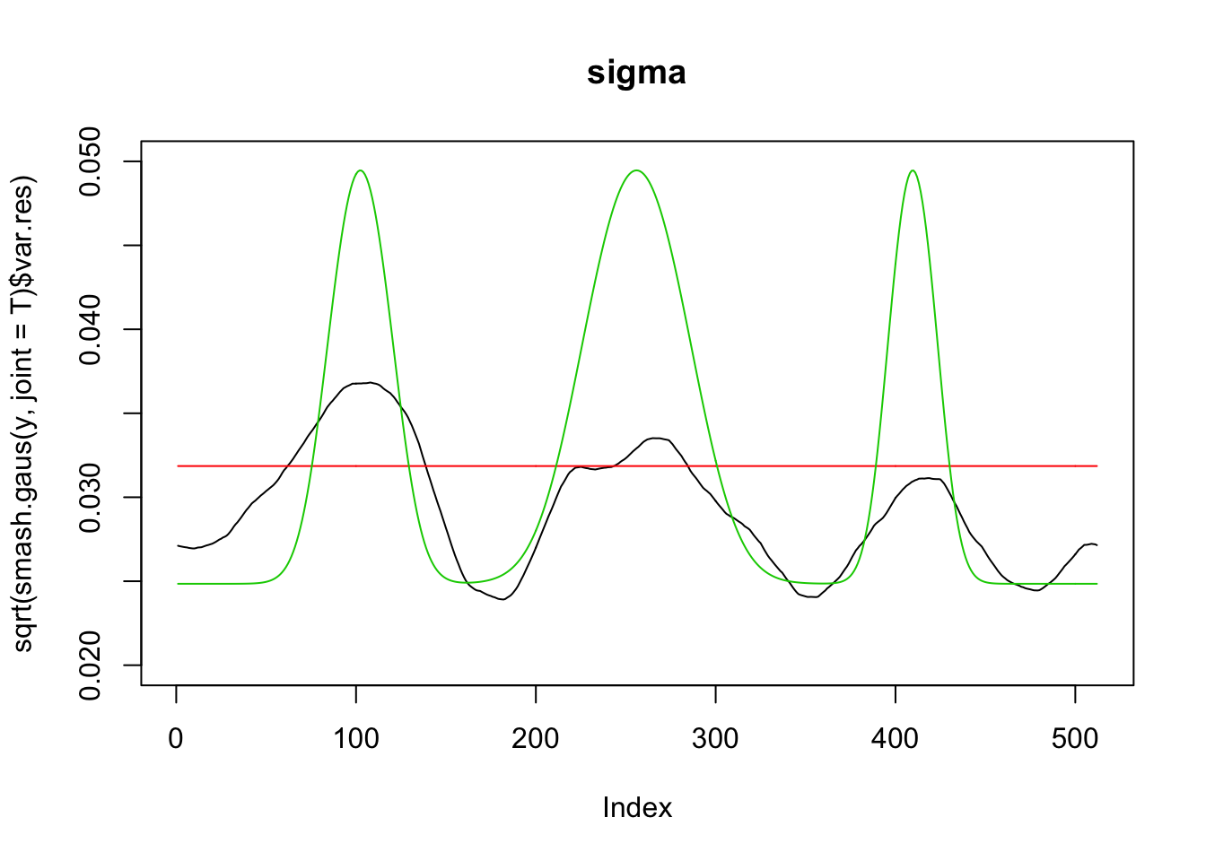
Expand here to see past versions of unnamed-chunk-2-2.png:
| Version | Author | Date |
|---|---|---|
| aacfc46 | Dongyue Xie | 2018-10-02 |
mean(sigma.t)[1] 0.03185823mean(sqrt(smash.gaus(y,joint=T)$var.res))[1] 0.02924347Decrease n to 256:
n = 64
t = 1:n/n
spike.f = function(x) (0.75 * exp(-500 * (x - 0.23)^2) +
            1.5  * exp(-2000 * (x - 0.33)^2) +
        3    * exp(-8000 * (x - 0.47)^2) +
            2.25 * exp(-16000 * (x - 0.69)^2) +
        0.5  * exp(-32000 * (x - 0.83)^2))
mu.s = spike.f(t)

# Scale the signal to be between 0.2 and 0.8.
mu.t = (1 + mu.s)/5
#plot(mu.t, type = "l",main='main function')

# Create the baseline variance function. (The function V2 from Cai &
# Wang 2008 is used here.)
var.fn = (1e-04 + 4 * (exp(-550 * (t - 0.2)^2) +
  exp(-200 * (t - 0.5)^2) + exp(-950 * (t - 0.8)^2)))/1.35+1
#plot(var.fn, type = "l")

# Set the signal-to-noise ratio.
rsnr = sqrt(3)
sigma.t = sqrt(var.fn)/mean(sqrt(var.fn)) * sd(mu.t)/rsnr^2

set.seed(12345)
y=mu.t+rnorm(n,0,sigma.t)
plot(y,col='grey80',main='n=256,SNR=3')
lines(smash.gaus(y))
lines(smash.gaus(y,mean(sigma.t)),col=2)
lines(smash.gaus(y,sigma.t),col=3)
lines(mu.t,col='grey80')
legend('topleft',c('smashu','smash.mean.sigma','smash.true.sigma','true mean'),col=c(1,2,3,'grey80'),lty=c(1,1,1,1))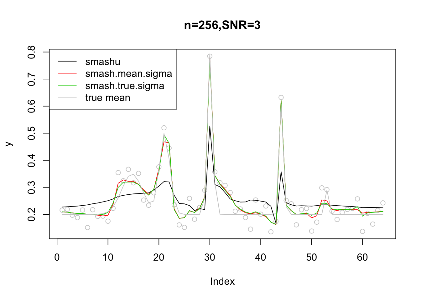
Expand here to see past versions of unnamed-chunk-3-1.png:
| Version | Author | Date |
|---|---|---|
| e7afb4d | Dongyue Xie | 2018-10-02 |
plot(sqrt(smash.gaus(y,joint=T)$var.res),type='l',ylim=c(0.01,0.08),main='sigma')
lines(rep(mean(sigma.t),n),col=2)
lines(sigma.t,col=3)
Expand here to see past versions of unnamed-chunk-3-2.png:
| Version | Author | Date |
|---|---|---|
| e7afb4d | Dongyue Xie | 2018-10-02 |
mean(sigma.t)[1] 0.03423118mean(sqrt(smash.gaus(y,joint=T)$var.res))[1] 0.07396342Decrease n to 64:
n = 64
t = 1:n/n
spike.f = function(x) (0.75 * exp(-500 * (x - 0.23)^2) +
            1.5  * exp(-2000 * (x - 0.33)^2) +
        3    * exp(-8000 * (x - 0.47)^2) +
            2.25 * exp(-16000 * (x - 0.69)^2) +
        0.5  * exp(-32000 * (x - 0.83)^2))
mu.s = spike.f(t)

# Scale the signal to be between 0.2 and 0.8.
mu.t = (1 + mu.s)/5
#plot(mu.t, type = "l",main='main function')

# Create the baseline variance function. (The function V2 from Cai &
# Wang 2008 is used here.)
var.fn = (1e-04 + 4 * (exp(-550 * (t - 0.2)^2) +
  exp(-200 * (t - 0.5)^2) + exp(-950 * (t - 0.8)^2)))/1.35+1
#plot(var.fn, type = "l")

# Set the signal-to-noise ratio.
rsnr = sqrt(3)
sigma.t = sqrt(var.fn)/mean(sqrt(var.fn)) * sd(mu.t)/rsnr^2

set.seed(12345)
y=mu.t+rnorm(n,0,sigma.t)
plot(y,col='grey80',main='n=64,SNR=3')
lines(smash.gaus(y))
lines(smash.gaus(y,mean(sigma.t)),col=2)
lines(smash.gaus(y,sigma.t),col=3)
lines(mu.t,col='grey80')
legend('topleft',c('smashu','smash.mean.sigma','smash.true.sigma','true mean'),col=c(1,2,3,'grey80'),lty=c(1,1,1,1))
Expand here to see past versions of unnamed-chunk-4-1.png:
| Version | Author | Date |
|---|---|---|
| e7afb4d | Dongyue Xie | 2018-10-02 |
plot(sqrt(smash.gaus(y,joint=T)$var.res),type='l',ylim=c(0.01,0.08),main='sigma')
lines(rep(mean(sigma.t),n),col=2)
lines(sigma.t,col=3)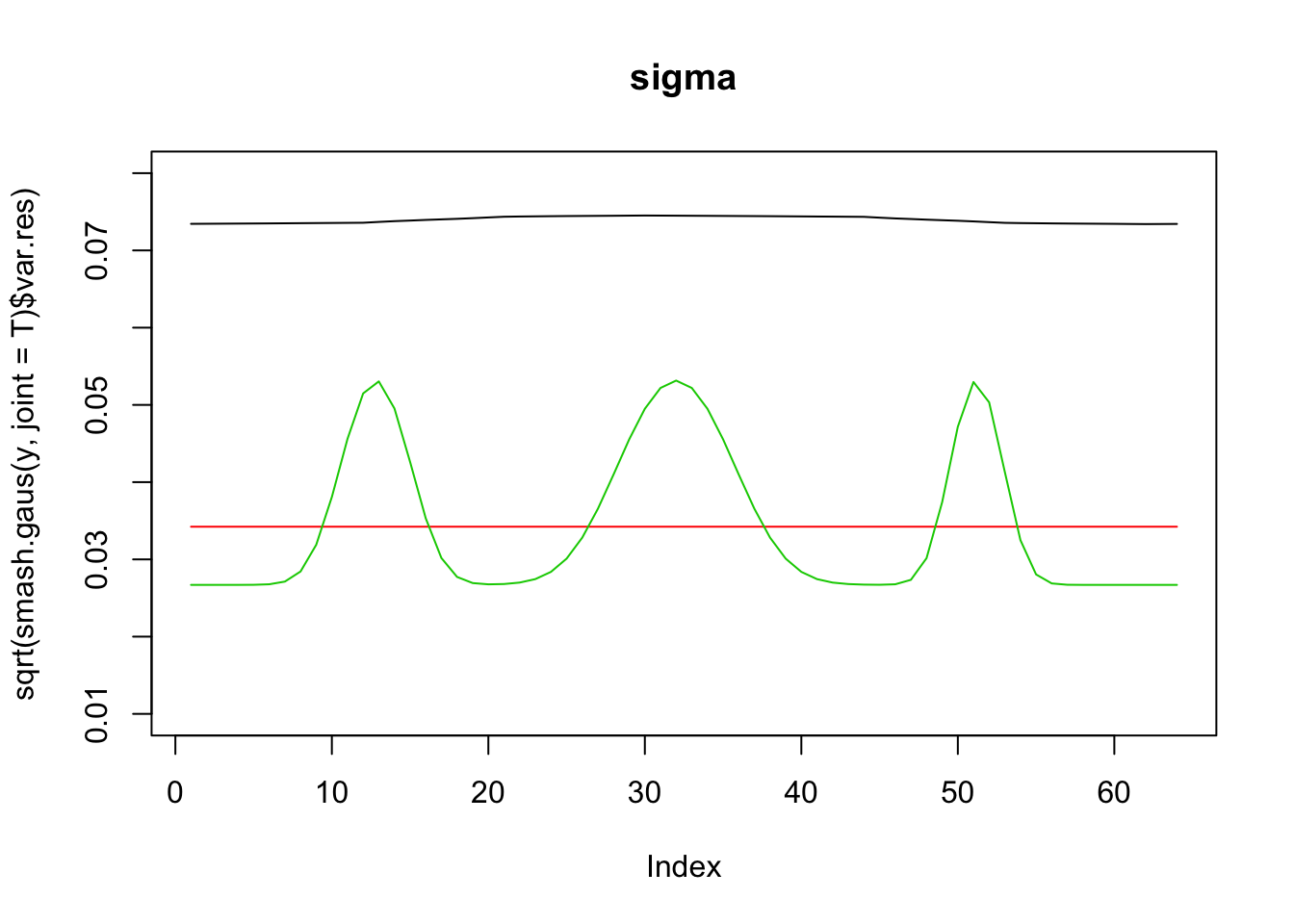
Expand here to see past versions of unnamed-chunk-4-2.png:
| Version | Author | Date |
|---|---|---|
| e7afb4d | Dongyue Xie | 2018-10-02 |
mean(sigma.t)[1] 0.03423118mean(sqrt(smash.gaus(y,joint=T)$var.res))[1] 0.07396342Decrease SNR:
n = 512
t = 1:n/n
spike.f = function(x) (0.75 * exp(-500 * (x - 0.23)^2) +
            1.5  * exp(-2000 * (x - 0.33)^2) +
        3    * exp(-8000 * (x - 0.47)^2) +
            2.25 * exp(-16000 * (x - 0.69)^2) +
        0.5  * exp(-32000 * (x - 0.83)^2))
mu.s = spike.f(t)

# Scale the signal to be between 0.2 and 0.8.
mu.t = (1 + mu.s)/5
#plot(mu.t, type = "l",main='main function')

# Create the baseline variance function. (The function V2 from Cai &
# Wang 2008 is used here.)
var.fn = (1e-04 + 4 * (exp(-550 * (t - 0.2)^2) +
  exp(-200 * (t - 0.5)^2) + exp(-950 * (t - 0.8)^2)))/1.35+1
#plot(var.fn, type = "l")

# Set the signal-to-noise ratio.
rsnr = sqrt(1)
sigma.t = sqrt(var.fn)/mean(sqrt(var.fn)) * sd(mu.t)/rsnr^2

set.seed(12345)
y=mu.t+rnorm(n,0,sigma.t)
plot(y,col='grey80',main='n=512,SNR=1')
lines(smash.gaus(y))
lines(smash.gaus(y,mean(sigma.t)),col=2)
lines(smash.gaus(y,sigma.t),col=3)
lines(mu.t,col='grey80')
legend('topleft',c('smashu','smash.mean.sigma','smash.true.sigma','true mean'),col=c(1,2,3,'grey80'),lty=c(1,1,1,1))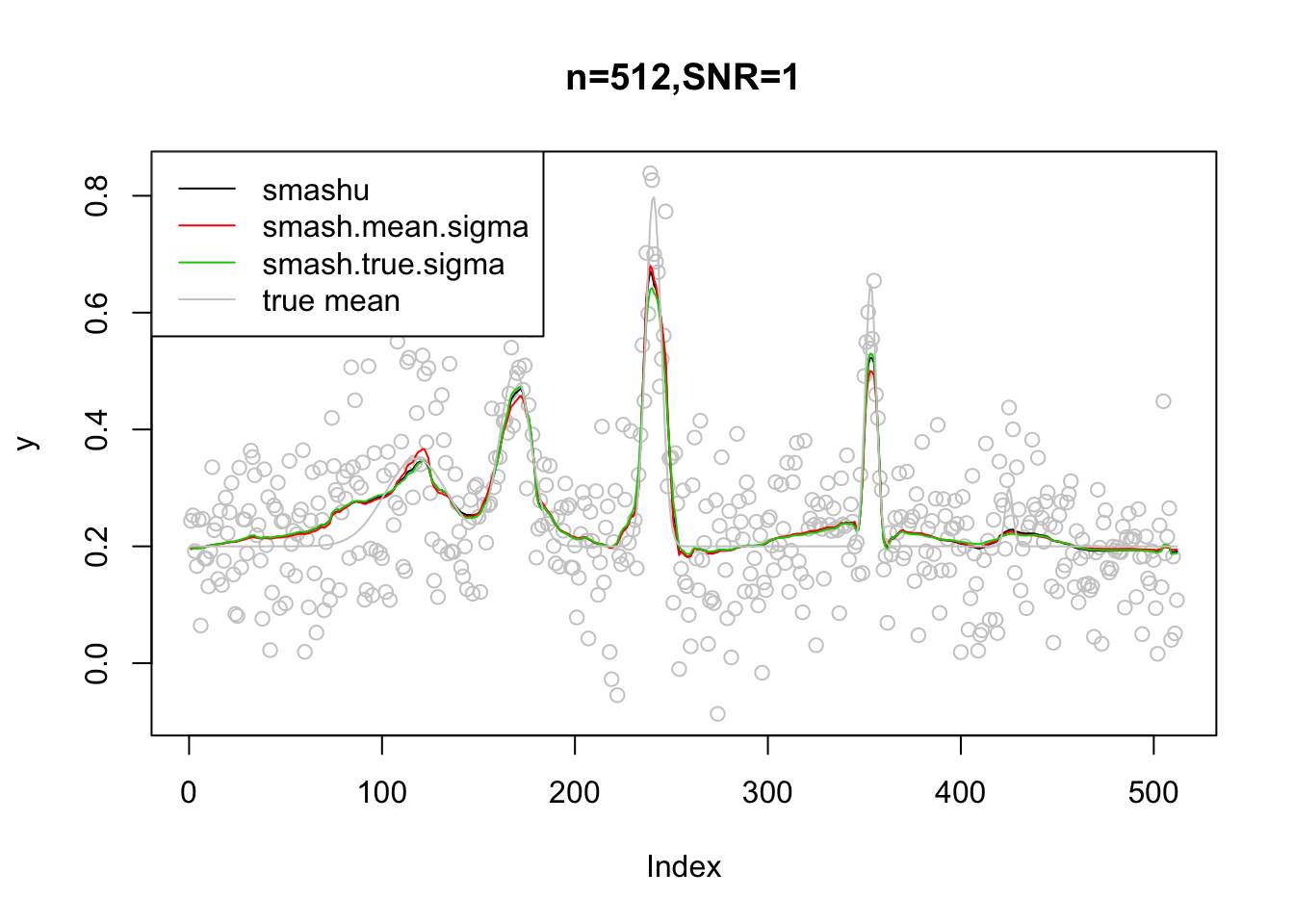
plot(sqrt(smash.gaus(y,joint=T)$var.res),type='l',ylim=c(0.07,0.15),main='sigma')
lines(rep(mean(sigma.t),n),col=2)
lines(sigma.t,col=3)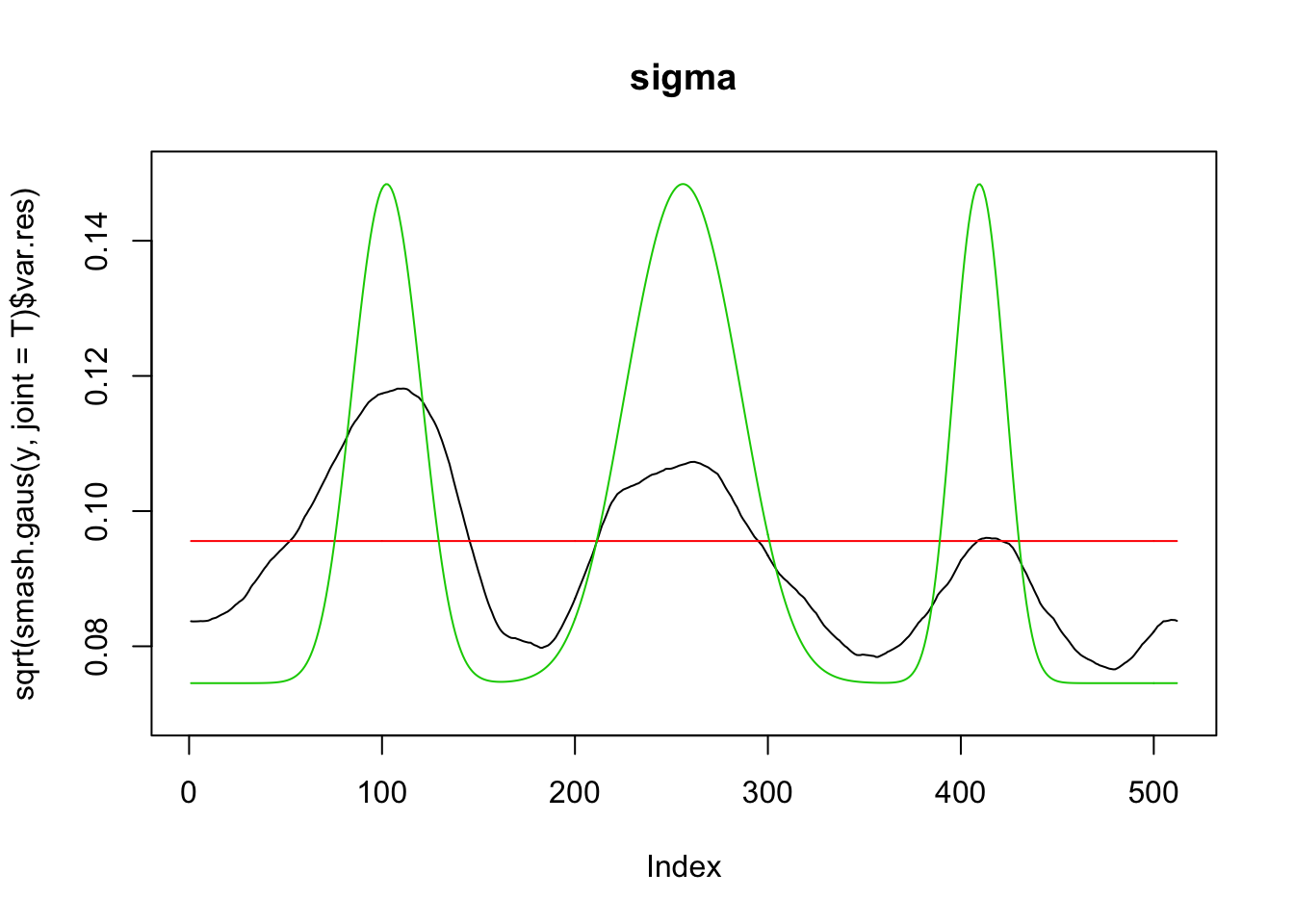
mean(sigma.t)[1] 0.0955747mean(sqrt(smash.gaus(y,joint=T)$var.res))[1] 0.09278895Summary
smash.gausis more sensitive to the scale of variance instead of the shape of variance.- As long as n is large enough so that smash can give good estimation of scale of variance and roughly satifactory shape, then
smash.gauscan still give similar mean estimation.
Session information
sessionInfo()R version 3.5.1 (2018-07-02)
Platform: x86_64-apple-darwin15.6.0 (64-bit)
Running under: macOS High Sierra 10.13.6
Matrix products: default
BLAS: /Library/Frameworks/R.framework/Versions/3.5/Resources/lib/libRblas.0.dylib
LAPACK: /Library/Frameworks/R.framework/Versions/3.5/Resources/lib/libRlapack.dylib
locale:
[1] en_US.UTF-8/en_US.UTF-8/en_US.UTF-8/C/en_US.UTF-8/en_US.UTF-8
attached base packages:
[1] stats graphics grDevices utils datasets methods base
other attached packages:
[1] smashr_1.2-0
loaded via a namespace (and not attached):
[1] Rcpp_0.12.18 knitr_1.20 whisker_0.3-2
[4] magrittr_1.5 workflowr_1.1.1 REBayes_1.3
[7] MASS_7.3-50 pscl_1.5.2 doParallel_1.0.14
[10] SQUAREM_2017.10-1 lattice_0.20-35 foreach_1.4.4
[13] ashr_2.2-7 stringr_1.3.1 caTools_1.17.1.1
[16] tools_3.5.1 parallel_3.5.1 grid_3.5.1
[19] data.table_1.11.6 R.oo_1.22.0 git2r_0.23.0
[22] iterators_1.0.10 htmltools_0.3.6 assertthat_0.2.0
[25] yaml_2.2.0 rprojroot_1.3-2 digest_0.6.17
[28] Matrix_1.2-14 bitops_1.0-6 codetools_0.2-15
[31] R.utils_2.7.0 evaluate_0.11 rmarkdown_1.10
[34] wavethresh_4.6.8 stringi_1.2.4 compiler_3.5.1
[37] Rmosek_8.0.69 backports_1.1.2 R.methodsS3_1.7.1
[40] truncnorm_1.0-8 This reproducible R Markdown analysis was created with workflowr 1.1.1