Estimate Null Correlation Problem
Yuxin Zou
2018-07-09
Last updated: 2018-08-13
library(mashr)Loading required package: ashrlibrary(knitr)
library(kableExtra)
source('../code/generateDataV.R')
source('../code/summary.R')We illustrate the problem about estimating the correlation matrix in mashr.
In my simple simulation, the current approach underestimates the null correlation. We need to find better positive definite estimator. We could try to estimate the pairwise correlation, ie. mle of \(\sum_{l,k} \pi_{lk} N_{2}(0, V + w_{l}U_{k})\) for any pair of conditions.
Simple simulation in \(R^2\) to illustrate the problem: \[ \hat{\beta}|\beta \sim N_{2}(\hat{\beta}; \beta, \left(\begin{matrix} 1 & 0.5 \\ 0.5 & 1 \end{matrix}\right)) \]
\[ \beta \sim \frac{1}{4}\delta_{0} + \frac{1}{4}N_{2}(0, \left(\begin{matrix} 1 & 0 \\ 0 & 0 \end{matrix}\right)) + \frac{1}{4}N_{2}(0, \left(\begin{matrix} 0 & 0 \\ 0 & 1 \end{matrix}\right)) + \frac{1}{4}N_{2}(0, \left(\begin{matrix} 1 & 1 \\ 1 & 1 \end{matrix}\right)) \]
\(\Rightarrow\) \[ \hat{\beta} \sim \frac{1}{4}N_{2}(0, \left( \begin{matrix} 1 & 0.5 \\ 0.5 & 1 \end{matrix} \right)) + \frac{1}{4}N_{2}(0, \left( \begin{matrix} 2 & 0.5 \\ 0.5 & 1 \end{matrix} \right)) + \frac{1}{4}N_{2}(0, \left( \begin{matrix} 1 & 0.5 \\ 0.5 & 2 \end{matrix} \right)) + \frac{1}{4}N_{2}(0, \left( \begin{matrix} 2 & 1.5 \\ 1.5 & 2 \end{matrix} \right)) \]
n = 4000
set.seed(1)
n = 4000; p = 2
Sigma = matrix(c(1,0.5,0.5,1),p,p)
U0 = matrix(0,2,2)
U1 = U0; U1[1,1] = 1
U2 = U0; U2[2,2] = 1
U3 = matrix(1,2,2)
Utrue = list(U0=U0, U1=U1, U2=U2, U3=U3)
data = generate_data(n, p, Sigma, Utrue)
Let’s check the result of mash under different correlation matrix:
- Identity \[ V.I = I_{2} \]
m.data = mash_set_data(data$Bhat, data$Shat)
U.c = cov_canonical(m.data)
m.I = mash(m.data, U.c, verbose= FALSE)- The truncated empirical correlation \(V.trun\)
Vhat = estimate_null_correlation(m.data, apply_lower_bound = FALSE)
Vhat
[,1] [,2]
[1,] 1.0000000 0.3439205
[2,] 0.3439205 1.0000000It underestimates the correlation.
# Use underestimate cor
m.data.V = mash_set_data(data$Bhat, data$Shat, V=Vhat)
m.V = mash(m.data.V, U.c, verbose = FALSE)- Overestimate correlation \[ V.o = \left( \begin{matrix} 1 & 0.65 \\ 0.65 & 1\end{matrix} \right) \]
# If we overestimate cor
V.o = matrix(c(1,0.65,0.65,1),2,2)
m.data.Vo = mash_set_data(data$Bhat, data$Shat, V=V.o)
m.Vo = mash(m.data.Vo, U.c, verbose=FALSE)- mash.1by1
We run ash for each condition, and estimate correlation matrix based on the non-significant genes. The estimated cor is closer to the truth.
m.1by1 = mash_1by1(m.data)
strong = get_significant_results(m.1by1)
V.mash = cor(data$Bhat[-strong,])
V.mash
[,1] [,2]
[1,] 1.0000000 0.4597745
[2,] 0.4597745 1.0000000m.data.1by1 = mash_set_data(data$Bhat, data$Shat, V=V.mash)
m.V1by1 = mash(m.data.1by1, U.c, verbose = FALSE)- True correlation
# With correct cor
m.data.correct = mash_set_data(data$Bhat, data$Shat, V=Sigma)
m.correct = mash(m.data.correct, U.c, verbose = FALSE)
The results are summarized in table:
null.ind = which(apply(data$B,1,sum) == 0)
V.trun = c(get_loglik(m.V), length(get_significant_results(m.V)), sum(get_significant_results(m.V) %in% null.ind))
V.I = c(get_loglik(m.I), length(get_significant_results(m.I)), sum(get_significant_results(m.I) %in% null.ind))
V.over = c(get_loglik(m.Vo), length(get_significant_results(m.Vo)), sum(get_significant_results(m.Vo) %in% null.ind))
V.1by1 = c(get_loglik(m.V1by1), length(get_significant_results(m.V1by1)), sum(get_significant_results(m.V1by1) %in% null.ind))
V.correct = c(get_loglik(m.correct), length(get_significant_results(m.correct)), sum(get_significant_results(m.correct) %in% null.ind))
temp = cbind(V.I, V.trun, V.1by1, V.correct, V.over)
colnames(temp) = c('Identity','truncate', 'm.1by1', 'true', 'overestimate')
row.names(temp) = c('log likelihood', '# significance', '# False positive')
temp %>% kable() %>% kable_styling()| Identity | truncate | m.1by1 | true | overestimate | |
|---|---|---|---|---|---|
| log likelihood | -12390.14 | -12307.65 | -12304.13 | -12302.62 | -12301.81 |
| # significance | 166.00 | 30.00 | 25.00 | 25.00 | 70.00 |
| # False positive | 14.00 | 1.00 | 0.00 | 0.00 | 4.00 |
The estimated pi is
par(mfrow=c(2,3))
barplot(get_estimated_pi(m.I), las=2, cex.names = 0.7, main='Identity', ylim=c(0,0.8))
barplot(get_estimated_pi(m.V), las=2, cex.names = 0.7, main='Truncate', ylim=c(0,0.8))
barplot(get_estimated_pi(m.V1by1), las=2, cex.names = 0.7, main='m.1by1', ylim=c(0,0.8))
barplot(get_estimated_pi(m.correct), las=2, cex.names = 0.7, main='True', ylim=c(0,0.8))
barplot(get_estimated_pi(m.Vo), las=2, cex.names = 0.7, main='OverEst', ylim=c(0,0.8))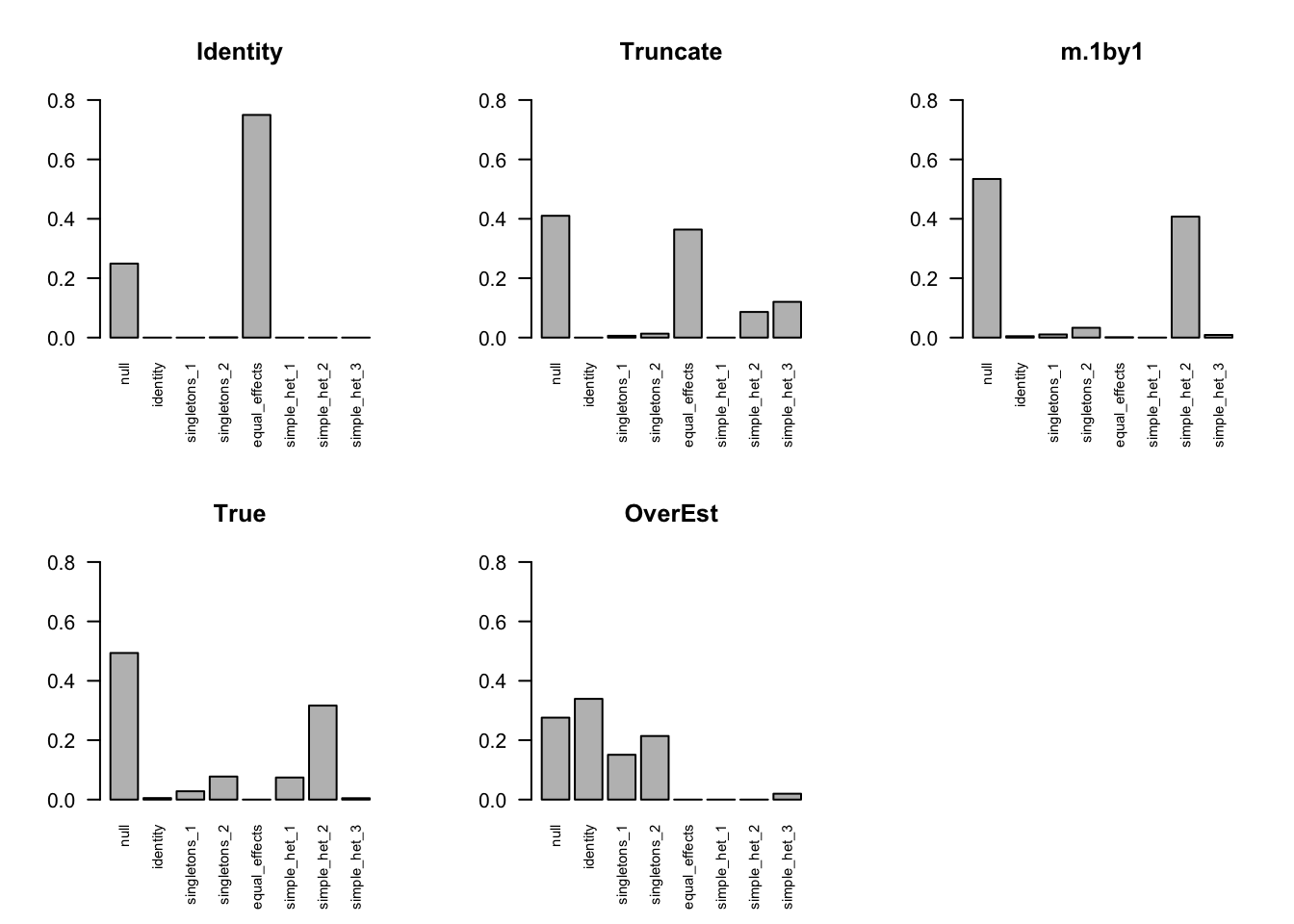
The ROC curve:
m.I.seq = ROC.table(data$B, m.I)
m.V.seq = ROC.table(data$B, m.V)
m.Vo.seq = ROC.table(data$B, m.Vo)
m.V1by1.seq = ROC.table(data$B, m.V1by1)
m.correct.seq = ROC.table(data$B, m.correct)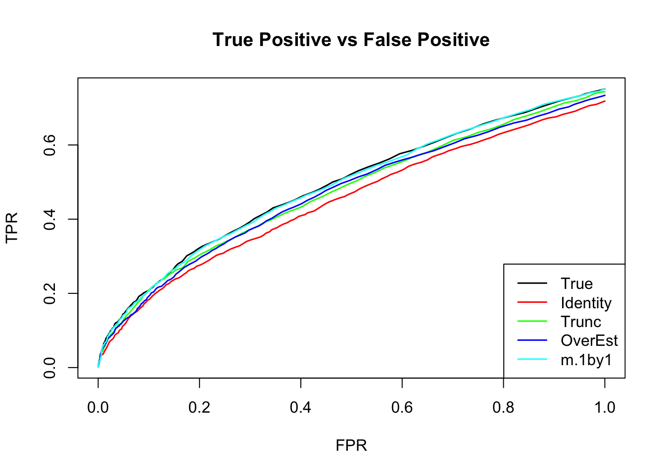
Comparing accuracy
rrmse = RRMSE(data$B, data$Bhat, list(m.I, m.V, m.V1by1, m.correct, m.Vo))
barplot(rrmse, ylim=c(0,(1+max(rrmse))/2), names.arg = c('Identity','V.trun','V.1by1','V.true','V.over'), las=2, cex.names = 0.7, main='RRMSE')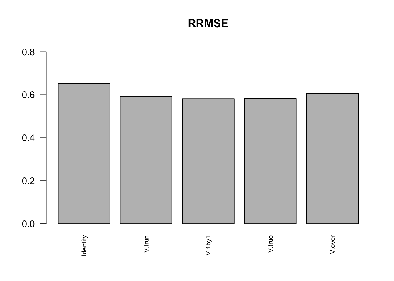
Solution: MLE
K=1
Suppose a simple extreme case \[ \left(\begin{matrix} \hat{x} \\ \hat{y} \end{matrix} \right)| \left(\begin{matrix} x \\ y \end{matrix} \right) \sim N_{2}(\left(\begin{matrix} \hat{x} \\ \hat{y} \end{matrix} \right); \left(\begin{matrix} x \\ y \end{matrix} \right), \left( \begin{matrix} 1 & \rho \\ \rho & 1 \end{matrix}\right)) \] \[ \left(\begin{matrix} x \\ y \end{matrix} \right) \sim \delta_{0} \] \(\Rightarrow\) \[ \left(\begin{matrix} \hat{x} \\ \hat{y} \end{matrix} \right) \sim N_{2}(\left(\begin{matrix} \hat{x} \\ \hat{y} \end{matrix} \right); \left(\begin{matrix} 0 \\ 0 \end{matrix} \right), \left( \begin{matrix} 1 & \rho \\ \rho & 1 \end{matrix}\right)) \]
\[ f(\hat{x},\hat{y}) = \prod_{i=1}^{n} \frac{1}{2\pi\sqrt{1-\rho^2}} \exp \{-\frac{1}{2(1-\rho^2)}\left[ \hat{x}_{i}^2 + \hat{y}_{i}^2 - 2\rho \hat{x}_{i}\hat{y}_{i}\right] \} \] The MLE of \(\rho\): \[ \begin{align*} l(\rho) &= -\frac{n}{2}\log(1-\rho^2) - \frac{1}{2(1-\rho^2)}\left( \sum_{i=1}^{n} x_{i}^2 + y_{i}^2 - 2\rho x_{i}y_{i} \right) \\ l(\rho)' &= \frac{n\rho}{1-\rho^2} - \frac{\rho}{(1-\rho^2)^2} \sum_{i=1}^{n} (x_{i}^2 + y_{i}^2) + \frac{\rho^2 + 1}{(1-\rho^2)^2} \sum_{i=1}^{n} x_{i}y_{i} = 0 \\ &= \rho^{3} - \rho^{2}\frac{1}{n}\sum_{i=1}^{n} x_{i}y_{i} - \left( 1- \frac{1}{n} \sum_{i=1}^{n} x_{i}^{2} + y_{i}^{2} \right) \rho - \frac{1}{n}\sum_{i=1}^{n} x_{i}y_{i} = 0 \\ l(\rho)'' &= \frac{n(\rho^2+1)}{(1-\rho^2)^2} - \frac{1}{2}\left( \frac{8\rho^2}{(1-\rho^2)^{3}} + \frac{2}{(1-\rho^2)^2} \right)\sum_{i=1}^{n}(x_{i}^2 + y_{i}^2) + \{ \left( \frac{8\rho^2}{(1-\rho^2)^{3}} + \frac{2}{(1-\rho^2)^2} \right)\rho + \frac{4\rho}{(1-\rho^2)^2} \}\sum_{i=1}^{n}x_{i}y_{i} \end{align*} \]
The log likelihood is not a concave function in general. The score function has either 1 or 3 real solutions.
Kendall and Stuart (1979) noted that at least one of the roots is real and lies in the interval [−1, 1]. However, it is possible that all three roots are real and in the admissible interval, in which case the likelihood can be evaluated at each root to determine the true maximum likelihood estimate.
I simulate the data with \(\rho=0.6\) and plot the loglikelihood function:
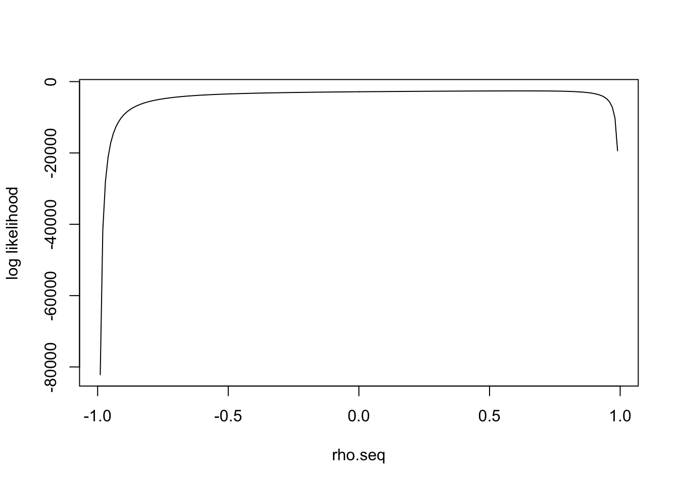
\(l(\rho)'\) has one real solution
polyroot(c(- sum(data$Bhat[,1]*data$Bhat[,2]), - (n - sum(data$Bhat[,1]^2 + data$Bhat[,2]^2)), - sum(data$Bhat[,1]*data$Bhat[,2]), n))[1] 0.6193031+0.000000i 0.0058209+1.009339i 0.0058209-1.009339iIn general
The general derivation is in estimate correlation mle
Session information
sessionInfo()R version 3.5.1 (2018-07-02)
Platform: x86_64-apple-darwin15.6.0 (64-bit)
Running under: macOS High Sierra 10.13.6
Matrix products: default
BLAS: /Library/Frameworks/R.framework/Versions/3.5/Resources/lib/libRblas.0.dylib
LAPACK: /Library/Frameworks/R.framework/Versions/3.5/Resources/lib/libRlapack.dylib
locale:
[1] en_US.UTF-8/en_US.UTF-8/en_US.UTF-8/C/en_US.UTF-8/en_US.UTF-8
attached base packages:
[1] stats graphics grDevices utils datasets methods base
other attached packages:
[1] kableExtra_0.9.0 knitr_1.20 mashr_0.2-11 ashr_2.2-10
loaded via a namespace (and not attached):
[1] Rcpp_0.12.18 highr_0.7 compiler_3.5.1
[4] pillar_1.3.0 plyr_1.8.4 iterators_1.0.10
[7] tools_3.5.1 digest_0.6.15 viridisLite_0.3.0
[10] evaluate_0.11 tibble_1.4.2 lattice_0.20-35
[13] pkgconfig_2.0.1 rlang_0.2.1 Matrix_1.2-14
[16] foreach_1.4.4 rstudioapi_0.7 yaml_2.2.0
[19] parallel_3.5.1 mvtnorm_1.0-8 xml2_1.2.0
[22] httr_1.3.1 stringr_1.3.1 REBayes_1.3
[25] hms_0.4.2 rprojroot_1.3-2 grid_3.5.1
[28] R6_2.2.2 rmarkdown_1.10 rmeta_3.0
[31] readr_1.1.1 magrittr_1.5 scales_0.5.0
[34] backports_1.1.2 codetools_0.2-15 htmltools_0.3.6
[37] MASS_7.3-50 rvest_0.3.2 assertthat_0.2.0
[40] colorspace_1.3-2 stringi_1.2.4 Rmosek_8.0.69
[43] munsell_0.5.0 pscl_1.5.2 doParallel_1.0.11
[46] truncnorm_1.0-8 SQUAREM_2017.10-1 crayon_1.3.4 This R Markdown site was created with workflowr