GTEx V6

Last updated: 2019-01-01

workflowr checks: (Click a bullet for more information)

✔ R Markdown file: up-to-date

Great! Since the R Markdown file has been committed to the Git repository, you know the exact version of the code that produced these results.
✔ Environment: empty

Great job! The global environment was empty. Objects defined in the global environment can affect the analysis in your R Markdown file in unknown ways. For reproduciblity it’s best to always run the code in an empty environment.
✔ Seed: set.seed(20181220)

The command set.seed(20181220) was run prior to running the code in the R Markdown file. Setting a seed ensures that any results that rely on randomness, e.g. subsampling or permutations, are reproducible.
✔ Session information: recorded

Great job! Recording the operating system, R version, and package versions is critical for reproducibility.
✔ Repository version: 26398fd
Great! You are using Git for version control. Tracking code development and connecting the code version to the results is critical for reproducibility. The version displayed above was the version of the Git repository at the time these results were generated.

Note that you need to be careful to ensure that all relevant files for the analysis have been committed to Git prior to generating the results (you can use wflow_publish or wflow_git_commit). workflowr only checks the R Markdown file, but you know if there are other scripts or data files that it depends on. Below is the status of the Git repository when the results were generated:
```
Ignored files:
    Ignored:    .DS_Store
    Ignored:    .Rhistory
    Ignored:    .Rproj.user/
    Ignored:    analysis/figure/
    Ignored:    output/.DS_Store

Untracked files:
    Untracked:  code/ED.R
    Untracked:  code/mCurrent.R
    Untracked:  code/mIgnore.R
    Untracked:  code/mMLE.R
    Untracked:  code/mSimple.R
    Untracked:  code/mV3.R
    Untracked:  data/cor_tissues_non_ash_voom_pearson.rda
    Untracked:  data/gene_names_GTEX_V6.txt
    Untracked:  data/genewide_ash_out_tissue_mat_halfuniform_non_mode.rda
    Untracked:  data/order_index.rda
    Untracked:  data/samples_id.txt
    Untracked:  data/tissuewide_pearson_halfuniform_tissuewide_non_mode.rda
    Untracked:  output/GTExV6/
```
Note that any generated files, e.g. HTML, png, CSS, etc., are not included in this status report because it is ok for generated content to have uncommitted changes.

Expand here to see past versions:

File	Version	Author	Date	Message
Rmd	26398fd	zouyuxin	2019-01-01	wflow_publish(“analysis/GTExV6.Rmd”)

library(flashr)
library(mixsqp)
library(mashr)

Loading required package: ashr

library(mclust)

Package 'mclust' version 5.4.1
Type 'citation("mclust")' for citing this R package in publications.


Attaching package: 'mclust'

The following object is masked from 'package:ashr':

    dens

library(knitr)
library(kableExtra)
library(ggplot2)

gtex <- readRDS(gzcon(url("https://github.com/stephenslab/gtexresults/blob/master/data/MatrixEQTLSumStats.Portable.Z.rds?raw=TRUE")))

strong.z = gtex$strong.z
data.strong = mash_set_data(strong.z)
data.random = mash_set_data(gtex$random.b, gtex$random.s)

Data Driven Covariances

Flash:

my_init_fn <- function(Y, K = 1) {
  ret = flashr:::udv_si(Y, K)
  pos_sum = sum(ret$v[ret$v > 0])
  neg_sum = -sum(ret$v[ret$v < 0])
  if (neg_sum > pos_sum) {
    return(list(u = -ret$u, d = ret$d, v = -ret$v))
  } else
    return(ret)
}

flash_pipeline = function(data, ...) {
  ## current state-of-the art
  ## suggested by Jason Willwerscheid
  ## cf: discussion section of
  ## https://willwerscheid.github.io/MASHvFLASH/MASHvFLASHnn2.html
  ebnm_fn = "ebnm_ash"
  ebnm_param = list(l = list(mixcompdist = "normal",
                             optmethod = "mixSQP"),
                    f = list(mixcompdist = "+uniform",
                             optmethod = "mixSQP"))
  ##
  fl_g <- flashr:::flash_greedy_workhorse(data,
                                          var_type = "constant",
                                          ebnm_fn = ebnm_fn,
                                          ebnm_param = ebnm_param,
                                          init_fn = "my_init_fn",
                                          stopping_rule = "factors",
                                          tol = 1e-3,
                                          verbose_output = "odF")
  fl_b <- flashr:::flash_backfit_workhorse(data,
                                           f_init = fl_g,
                                           var_type = "constant",
                                           ebnm_fn = ebnm_fn,
                                           ebnm_param = ebnm_param,
                                           stopping_rule = "factors",
                                           tol = 1e-3,
                                           verbose_output = "odF")
  return(fl_b)
}


cov_flash = function(data, subset = NULL, non_canonical = FALSE, save_model = NULL) {
  if(is.null(subset)) subset = 1:mashr:::n_effects(data)
  b.center = apply(data$Bhat, 2, function(x) x - mean(x))
  ## Only keep factors with at least two values greater than 1 / sqrt(n)
  find_nonunique_effects <- function(fl) {
    thresh <- 1/sqrt(ncol(fl$fitted_values))
    vals_above_avg <- colSums(fl$ldf$f > thresh)
    nonuniq_effects <- which(vals_above_avg > 1)
    return(fl$ldf$f[, nonuniq_effects, drop = FALSE])
  }
  fmodel = flash_pipeline(b.center)
  if (non_canonical)
    flash_f = find_nonunique_effects(fmodel)
  else 
    flash_f = fmodel$ldf$f
  ## row.names(flash_f) = colnames(b)
  if (!is.null(save_model)) saveRDS(list(model=fmodel, factors=flash_f), save_model)
  if(ncol(flash_f) == 0){
    U.flash = list("tFLASH" = t(fmodel$fitted_values) %*% fmodel$fitted_values / nrow(fmodel$fitted_values))
  } else{
    U.flash = c(cov_from_factors(t(as.matrix(flash_f)), "FLASH"),
  list("tFLASH" = t(fmodel$fitted_values) %*% fmodel$fitted_values / nrow(fmodel$fitted_values)))
  }
  
  return(U.flash)
}

U.f = cov_flash(data.strong, non_canonical = TRUE, save_model = '../output/GTExV6/flash_model.rds')
saveRDS(U.f, 'output/GTExV6/flash_cov.rds')

missing.tissues <- c(7, 8, 19, 20, 24, 25, 31, 34, 37)
gtex.colors <- read.table("https://github.com/stephenslab/gtexresults/blob/master/data/GTExColors.txt?raw=TRUE", sep = '\t', comment.char = '')[-missing.tissues, 2]
gtex.colors <- as.character(gtex.colors)

fl_model = readRDS('output/GTExV6/flash_model.rds')$model
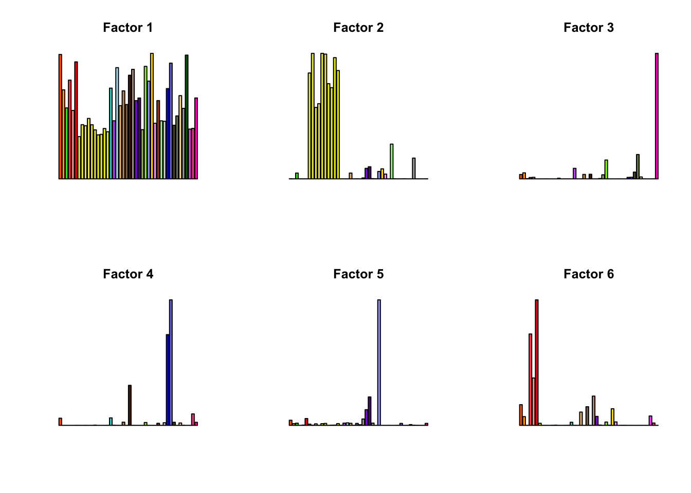
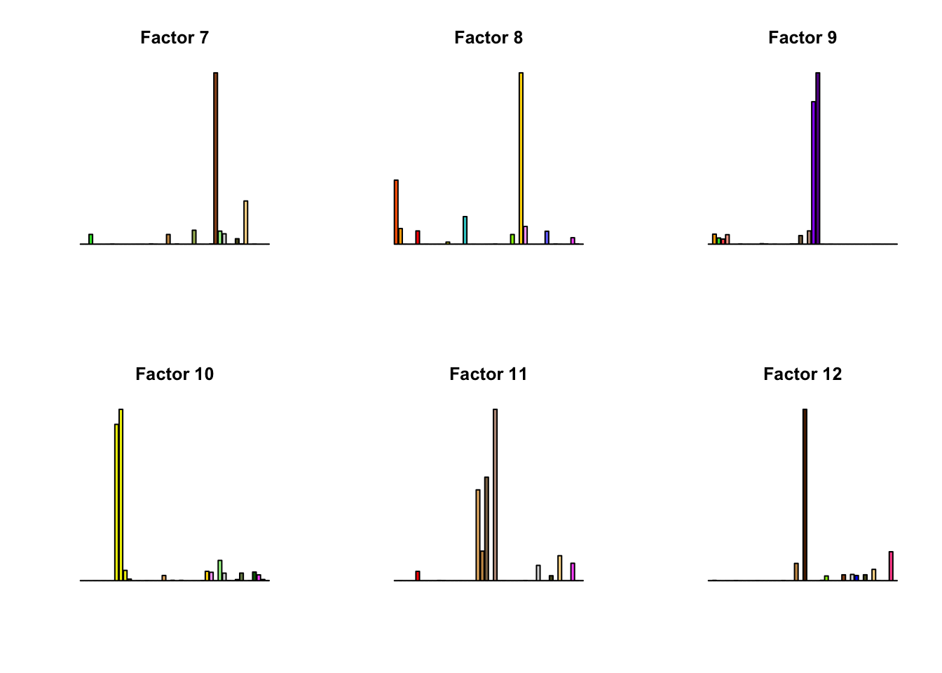
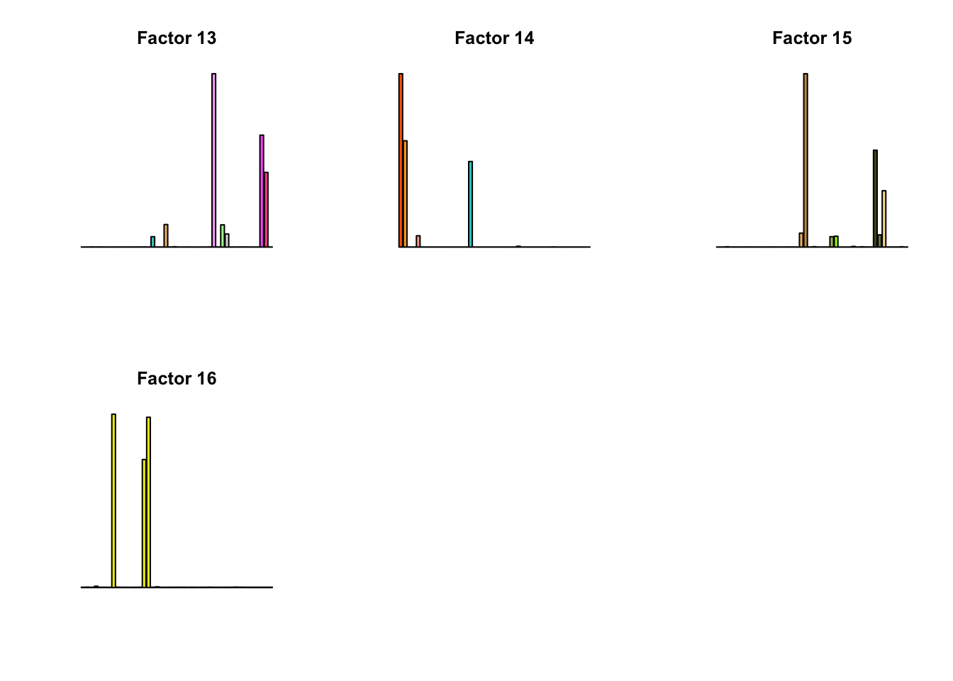
factors = readRDS('output/GTExV6/flash_model.rds')$factors
par(mfrow = c(2, 3))
for(k in 1:16){
  barplot(factors[,k], col=gtex.colors, names.arg = FALSE, axes = FALSE, main=paste0("Factor ", k))
}

fll_model = flash_pipeline(fl_model$ldf$l)
saveRDS(fll_model, 'output/GTExV6/flash_loading_model.rds')

U.pca = cov_pca(data.strong, 5)

U.ed = cov_ed(data.strong, c(U.f, U.pca))

U.ed = readRDS('output/GTExV6/Ued.rds')

U.c = cov_canonical(data.random)

data.strong = mash_set_data(Bhat = gtex$strong.b, Shat = gtex$strong.s)

m.ignore = mash(data.random, c(U.c, U.ed), outputlevel = 1)
m.ignore$result = mash_compute_posterior_matrices(m.ignore, data.strong)

V.simple = estimate_null_correlation_simple(data.random)

data.random.V.simple = mash_update_data(data.random, V = V.simple)
m.simple = mash(data.random.V.simple, c(U.c, U.ed), outputlevel = 1)
data.strong.V.simple = mash_update_data(data.strong, V = V.simple)
m.simple$result = mash_compute_posterior_matrices(m.simple, data.strong.V.simple)

set.seed(1)
random.subset = sample(1:nrow(gtex$random.b),5000)
data.random.s = mash_set_data(gtex$random.b[random.subset,], gtex$random.s[random.subset,])
current = estimate_null_correlation(data.random.s, c(U.c, U.ed), max_iter = 6)
V.current = current$V
data.random.V.current = mash_update_data(data.random, V = V.current)
m.current = mash(data.random.V.current, c(U.c, U.ed), outputlevel = 1)
data.strong = mash_update_data(data.strong, V = V.current)
m.current$result = mash_compute_posterior_matrices(m.current, data.strong)

V = get(load('~/Documents/GitHub/GTEx/data/genewide_ash_out_tissue_mat_halfuniform_non_mode.rda'))
# select tissue
tissue_labels <- read.table(file = "~/Documents/GitHub/GTEx/data/samples_id.txt")[,3]
U <- unique(tissue_labels)
tissues = c(1:6, 9:18, 21:23,26:30,32:33,35:36,38:53)
V = V[tissues,tissues,]

V.strong = V
for(i in 1:nrow(gtex$strong.b)){
  V.strong[,,i] = as.matrix(Matrix::nearPD(V[,,i], conv.tol=1.e-05, corr = TRUE, maxit = 200, doSym = TRUE)$mat)
}
saveRDS(V.strong, 'output/GTExV6/V_strong_genewide.rds')

# select genes
gene_names <- as.character(read.table(file = "~/Documents/GitHub/GTEx/data/gene_names_GTEX_V6.txt")[,1])
gene_names_1 <- as.character(sapply(gene_names, function(x) return(strsplit(x, "[.]")[[1]][1])))

data.random.names = rownames(data.random$Bhat)
data.random.names.1 = as.character(sapply(data.random.names, function(x) return(strsplit(x, "[.]")[[1]][1])))

V.random = array(NA, dim = c(44,44,nrow(gtex$random.b)))
for(i in 1:nrow(gtex$random.b)){
  numg <- grep(data.random.names.1[i], gene_names_1)
  V.random[,,i] = as.matrix(Matrix::nearPD(V[,,numg], conv.tol=1.e-05, corr = TRUE, doSym = TRUE)$mat)
}
saveRDS(V.random, 'output/GTExV6/V_random_genewide.rds')

data.random.V3 = mash_update_data(data.random, V = V.random)
m.V3 = mash(data.random.V3, c(U.c, U.ed), outputlevel = 1, algorithm.version = 'R')
data.strong.V3 = mash_update_data(data.strong, V = V.strong)
m.V3$result = mash_compute_posterior_matrices(m.V3, data.strong.V3, algorithm.version = 'R')

# read model
m_ignore = readRDS('output/GTExV6/m_ignore_post.rds')
m_ignore_EZ = readRDS('output/GTExV6/m_ignore_EZ_post.rds')
m_simple = readRDS('output/GTExV6/m_simple_post.rds')
m_simple_EZ = readRDS('output/GTExV6/m_simple_EZ_post.rds')
m_current = readRDS('output/GTExV6/m_current_post.rds')
m_current_EZ = readRDS('output/GTExV6/m_current_EZ_post.rds')
m_V3 = readRDS('output/GTExV6/m_V3_genewide_post.rds')
m_V3_EZ = readRDS('output/GTExV6/m_V3_genewide_EZ_post.rds')

par(mfrow = c(1,2))
# pdf('../output/GTExV6/Figures/SimpleV.pdf')
corrplot::corrplot(V.simple, method='color', type='upper', tl.col="black", tl.srt=45, tl.cex = 0.7, diag = FALSE, col=colorRampPalette(c("blue", "white", "red"))(200), cl.lim = c(-1,1), title = 'Simple', mar=c(0,0,5,0))

Warning in corrplot::corrplot(V.simple, method = "color", type = "upper", :
Not been able to calculate text margin, please try again with a clean new
empty window using {plot.new(); dev.off()} or reduce tl.cex

# dev.off()

V.current = readRDS('output/GTExV6/currentV_EZ.rds')
V.current = V.current$V
# pdf('../output/GTExV6/Figures/CurrentEZV.pdf')
corrplot::corrplot(V.current, method='color', type='upper', tl.col="black", tl.srt=45, tl.cex = 0.7, diag = FALSE, col=colorRampPalette(c("blue", "white", "red"))(200), cl.lim = c(-1,1), title = 'Current EZ', mar=c(0,0,5,0))

Warning in corrplot::corrplot(V.current, method = "color", type =
"upper", : Not been able to calculate text margin, please try again with a
clean new empty window using {plot.new(); dev.off()} or reduce tl.cex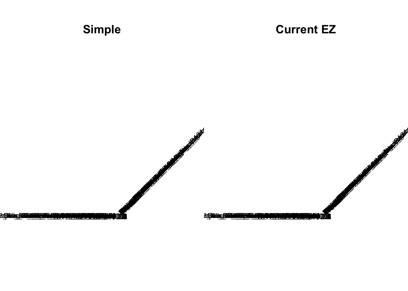

# dev.off()

logliks = c(get_loglik(m_ignore), get_loglik(m_simple), get_loglik(m_current), get_loglik(m_V3))
logliks_EZ = c(get_loglik(m_ignore_EZ), get_loglik(m_simple_EZ), get_loglik(m_current_EZ), get_loglik(m_V3_EZ))
tmp = cbind(logliks, logliks_EZ)
row.names(tmp) = c('Ignore', 'Simple', 'Current', 'V3')
colnames(tmp) = c('EE', 'EZ')
tmp %>% kable() %>% kable_styling()

	EE	EZ
Ignore	929188.2	935288.4
Simple	933359.2	936783.2
Current	937323.7	939685.2
V3	860927.1	897029.6

barplot(get_estimated_pi(m_ignore), las=2, cex.names = 0.7, main = 'Ignore EE')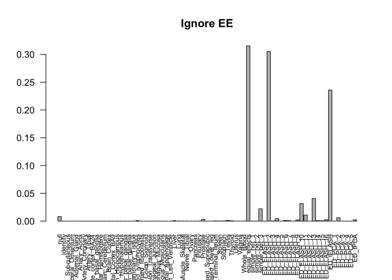

barplot(get_estimated_pi(m_simple), las=2, cex.names = 0.7, main = 'Simple EE')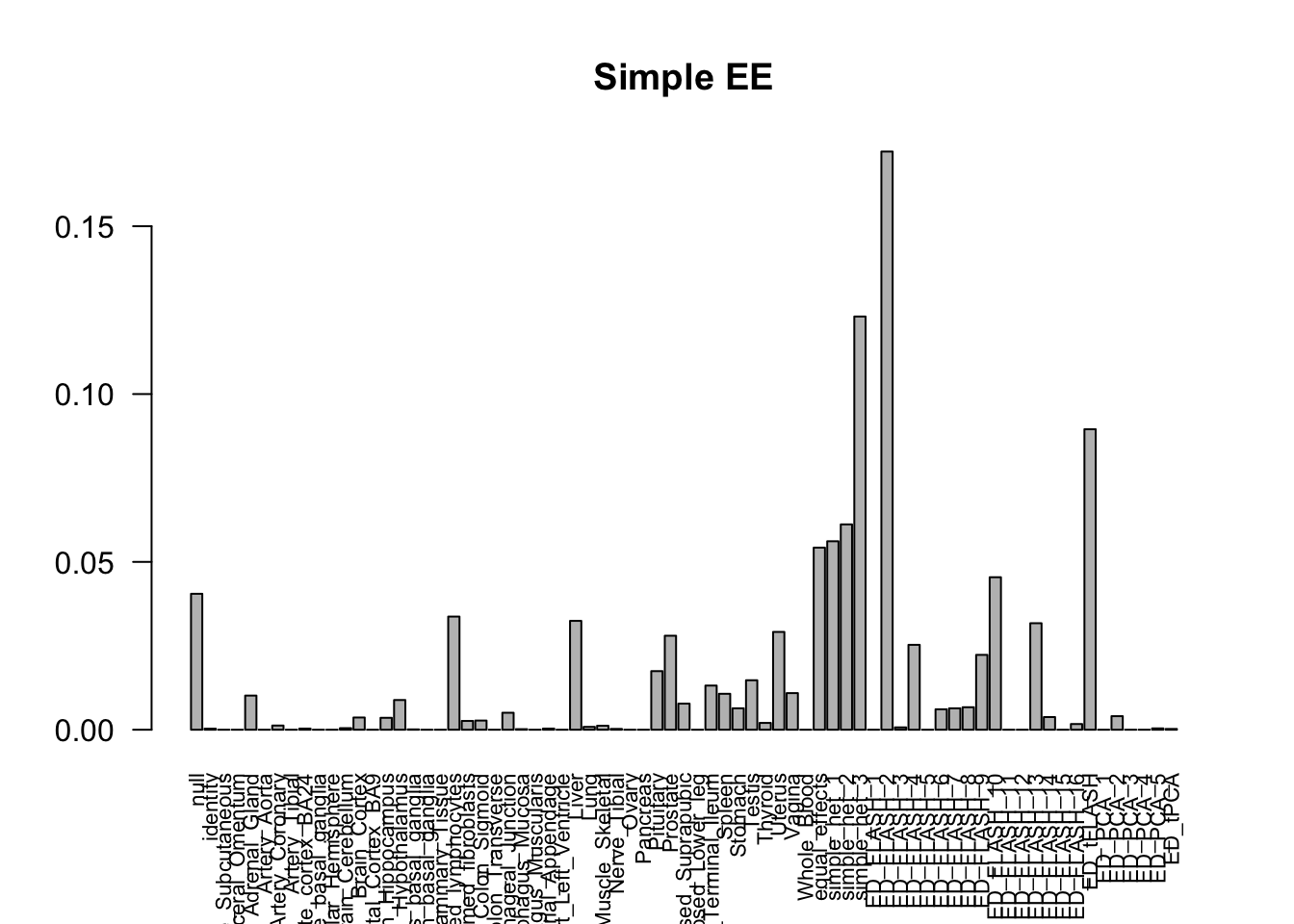

barplot(get_estimated_pi(m_current), las=2, cex.names = 0.7, main = 'Current EE')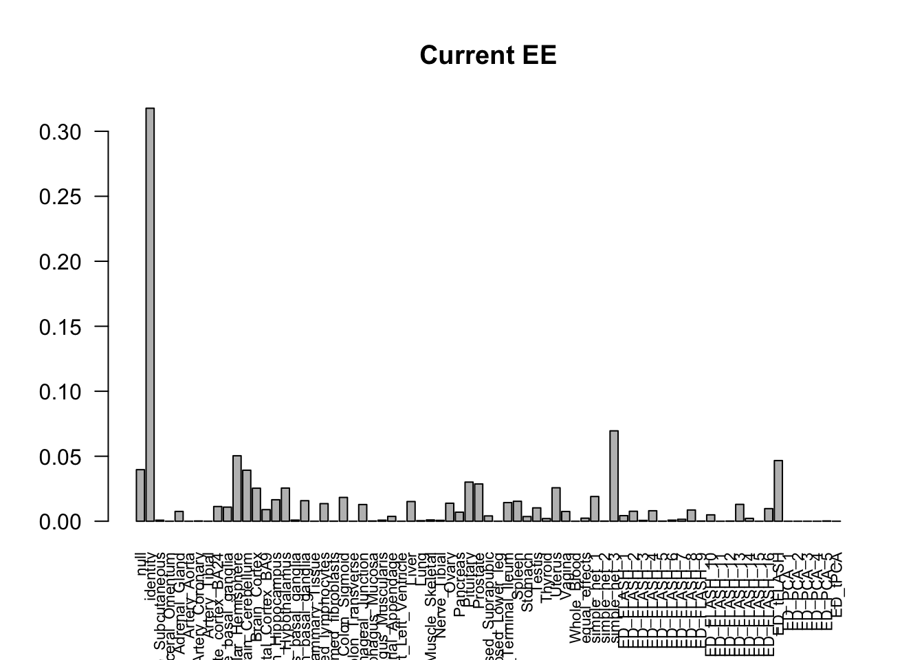

barplot(get_estimated_pi(m_V3), las=2, cex.names = 0.7, main = 'V3 EE')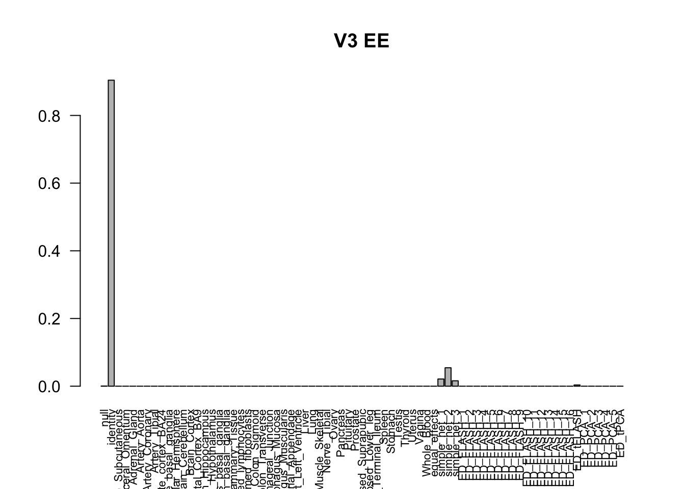

barplot(get_estimated_pi(m_ignore_EZ), las=2, cex.names = 0.7, main = 'Ignore EZ')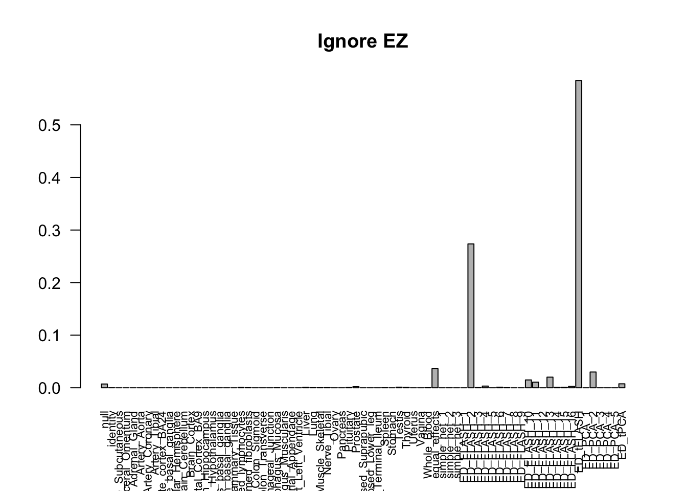

barplot(get_estimated_pi(m_simple_EZ), las=2, cex.names = 0.7, main = 'Simple EZ')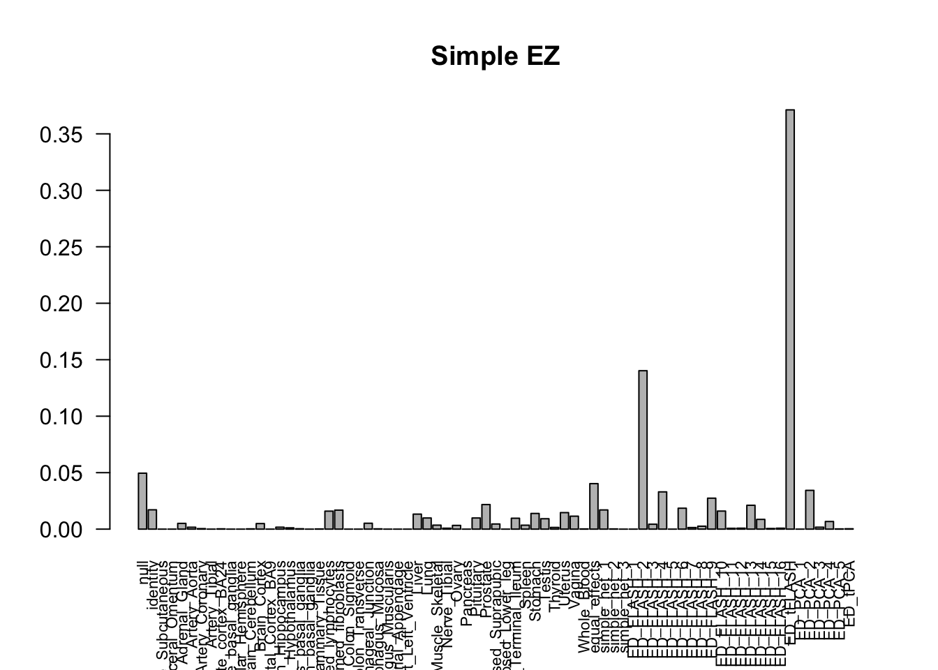

barplot(get_estimated_pi(m_current_EZ), las=2, cex.names = 0.7, main = 'Current EZ')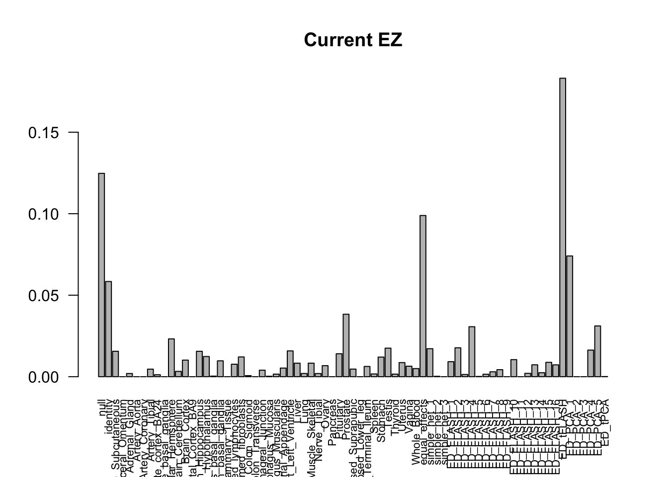

barplot(get_estimated_pi(m_V3_EZ), las=2, cex.names = 0.7, main = 'V3 EZ')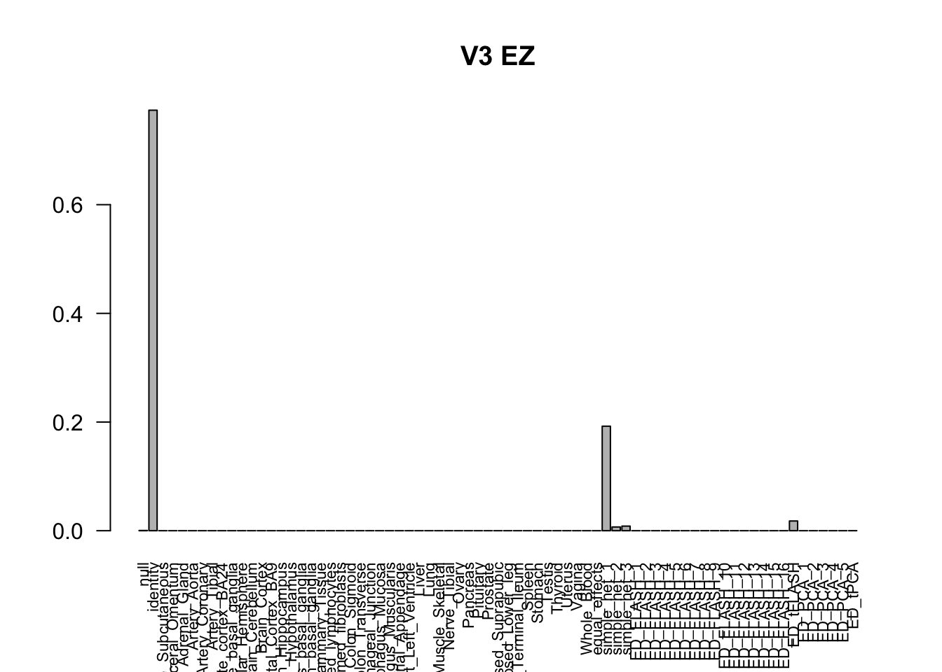

Number of significant:

numsig_EE = c(length(get_significant_results(m_ignore)), 
              length(get_significant_results(m_simple)), 
              length(get_significant_results(m_current)), 
              length(get_significant_results(m_V3)))
numsig_EZ = c(length(get_significant_results(m_ignore_EZ)), 
              length(get_significant_results(m_simple_EZ)), 
              length(get_significant_results(m_current_EZ)), 
              length(get_significant_results(m_V3_EZ)))
tmp = cbind(numsig_EE, numsig_EZ)
row.names(tmp) = c('Ignore', 'Simple', 'Current', 'V3')
colnames(tmp) = c('EE', 'EZ')
tmp %>% kable() %>% kable_styling()

	EE	EZ
Ignore	14017	14221
Simple	13037	13485
Current	12803	13006
V3	16054	16069

The V3 model has more significant findings, which includes all significant findings in the other three models.

length(intersect(get_significant_results(m_V3_EZ), get_significant_results(m_current_EZ)))

[1] 13006

length(intersect(get_significant_results(m_V3_EZ), get_significant_results(m_simple_EZ)))

[1] 13485

length(intersect(get_significant_results(m_V3_EZ), get_significant_results(m_ignore_EZ)))

[1] 14221

The gene significant in simple EZ, not in current EZ:

par(mfrow=c(2,2))
stronggene = data.frame(gtex$strong.b[5034,])
colnames(stronggene) = 'EffectSize'
stronggene$Group = row.names(stronggene)
stronggene$se = gtex$strong.s[5034,]
ggplot(stronggene, aes(y = EffectSize, x = Group)) + 
  geom_point(show.legend = FALSE, color=gtex.colors) + coord_flip() + ggtitle('ENSG00000135315') + ylim(c(-0.7,1)) + geom_errorbar(aes(ymin=EffectSize-1.96*se, ymax=EffectSize+1.96*se), width=0.4, show.legend = FALSE, color=gtex.colors) + 
  theme_bw(base_size=12) + theme(axis.text.y = element_text(colour = gtex.colors, size = 6))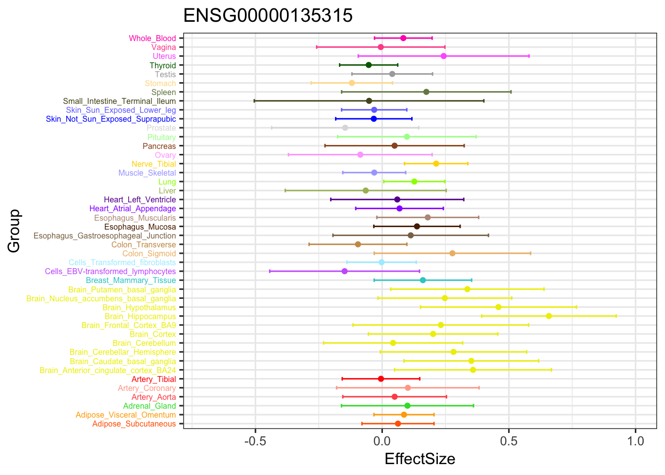

stronggeneSimple = data.frame(m_simple_EZ$result$PosteriorMean[5034,])
colnames(stronggeneSimple) = 'EffectSize'
stronggeneSimple$Group = row.names(stronggeneSimple)
stronggeneSimple$se = m_simple_EZ$result$PosteriorSD[5034,]
ggplot(stronggeneSimple, aes(y = EffectSize, x = Group)) + 
  geom_point(show.legend = FALSE, color=gtex.colors) + coord_flip() + ggtitle('ENSG00000135315 Simple') + ylim(c(-0.7,1)) + 
  geom_errorbar(aes(ymin=EffectSize-1.96*se, ymax=EffectSize+1.96*se), width=0.4, show.legend = FALSE, color=gtex.colors) + 
  theme_bw(base_size=12) + theme(axis.text.y = element_text(colour = gtex.colors, size = 6))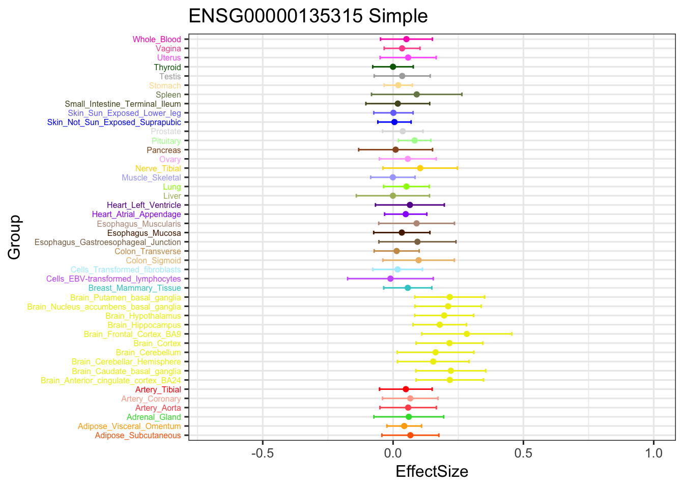

stronggeneCurrent = data.frame(m_current_EZ$result$PosteriorMean[5034,])
colnames(stronggeneCurrent) = 'EffectSize'
stronggeneCurrent$Group = row.names(stronggeneCurrent)
stronggeneCurrent$se = m_current_EZ$result$PosteriorSD[5034,]
ggplot(stronggeneCurrent, aes(y = EffectSize, x = Group)) + 
  geom_point(show.legend = FALSE, color=gtex.colors) + ylim(c(-0.7,1)) + coord_flip() + ggtitle('ENSG00000135315 Current') + 
  geom_errorbar(aes(ymin=EffectSize-1.96*se, ymax=EffectSize+1.96*se), width=0.4, show.legend = FALSE, color=gtex.colors) + 
  theme_bw(base_size=12) + theme(axis.text.y = element_text(colour = gtex.colors, size = 6))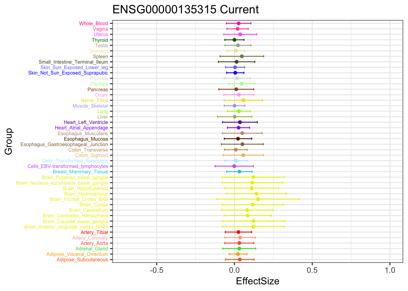

stronggeneV3 = data.frame(m_V3_EZ$result$PosteriorMean[5034,])
colnames(stronggeneV3) = 'EffectSize'
stronggeneV3$Group = row.names(stronggeneV3)
stronggeneV3$se = m_V3_EZ$result$PosteriorSD[5034,]
ggplot(stronggeneV3, aes(y = EffectSize, x = Group)) + 
  geom_point(show.legend = FALSE, color=gtex.colors) + ylim(c(-0.7,1)) + coord_flip() + ggtitle('ENSG00000135315 V3') + 
  geom_errorbar(aes(ymin=EffectSize-1.96*se, ymax=EffectSize+1.96*se), width=0.4, show.legend = FALSE, color=gtex.colors) + 
  theme_bw(base_size=12) + theme(axis.text.y = element_text(colour = gtex.colors, size = 6))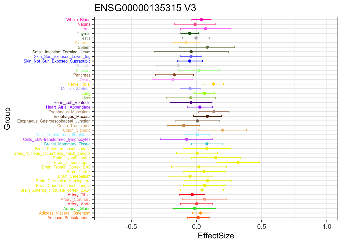

The gene MCPH1:

par(mfrow=c(1,3))
stronggene = data.frame(gtex$strong.b[13837,])
colnames(stronggene) = 'EffectSize'
stronggene$Group = row.names(stronggene)
stronggene$se = gtex$strong.s[13837,]
ggplot(stronggene, aes(y = EffectSize, x = Group)) + 
  geom_point(show.legend = FALSE, color=gtex.colors) + coord_flip() + ggtitle('ENSG00000249898') + ylim(c(-1.3,1.1)) + geom_errorbar(aes(ymin=EffectSize-1.96*se, ymax=EffectSize+1.96*se), width=0.4, show.legend = FALSE, color=gtex.colors) + 
  theme_bw(base_size=12) + theme(axis.text.y = element_text(colour = gtex.colors, size = 6))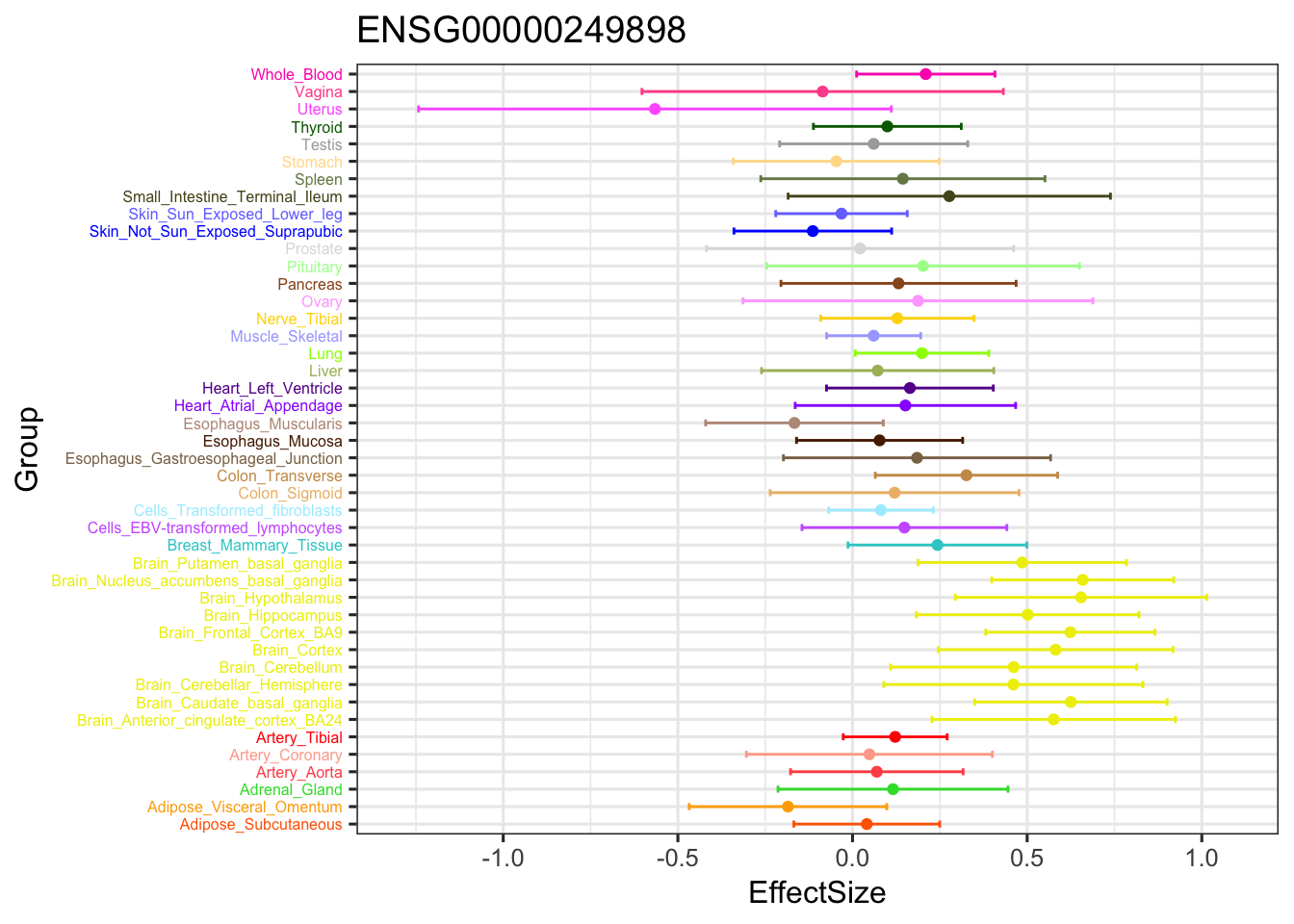

stronggeneCurrent = data.frame(m_current_EZ$result$PosteriorMean[13837,])
colnames(stronggeneCurrent) = 'EffectSize'
stronggeneCurrent$Group = row.names(stronggeneCurrent)
stronggeneCurrent$se = m_current_EZ$result$PosteriorSD[13837,]
ggplot(stronggeneCurrent, aes(y = EffectSize, x = Group)) + 
  geom_point(show.legend = FALSE, color=gtex.colors) + coord_flip() + ggtitle('ENSG00000249898 Current') + ylim(c(-1.3,1.1)) + 
  geom_errorbar(aes(ymin=EffectSize-1.96*se, ymax=EffectSize+1.96*se), width=0.4, show.legend = FALSE, color=gtex.colors) + 
  theme_bw(base_size=12) + theme(axis.text.y = element_text(colour = gtex.colors, size = 6))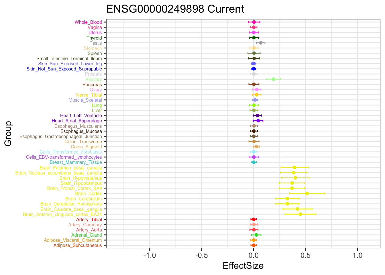

stronggeneV3 = data.frame(m_V3_EZ$result$PosteriorMean[13837,])
colnames(stronggeneV3) = 'EffectSize'
stronggeneV3$Group = row.names(stronggeneV3)
stronggeneV3$se = m_V3_EZ$result$PosteriorSD[13837,]
ggplot(stronggeneV3, aes(y = EffectSize, x = Group)) + 
  geom_point(show.legend = FALSE, color=gtex.colors) + ylim(c(-1.3,1.1)) + coord_flip() + ggtitle('ENSG00000249898 V3') + 
  geom_errorbar(aes(ymin=EffectSize-1.96*se, ymax=EffectSize+1.96*se), width=0.4, show.legend = FALSE, color=gtex.colors) + 
  theme_bw(base_size=12) + theme(axis.text.y = element_text(colour = gtex.colors, size = 6))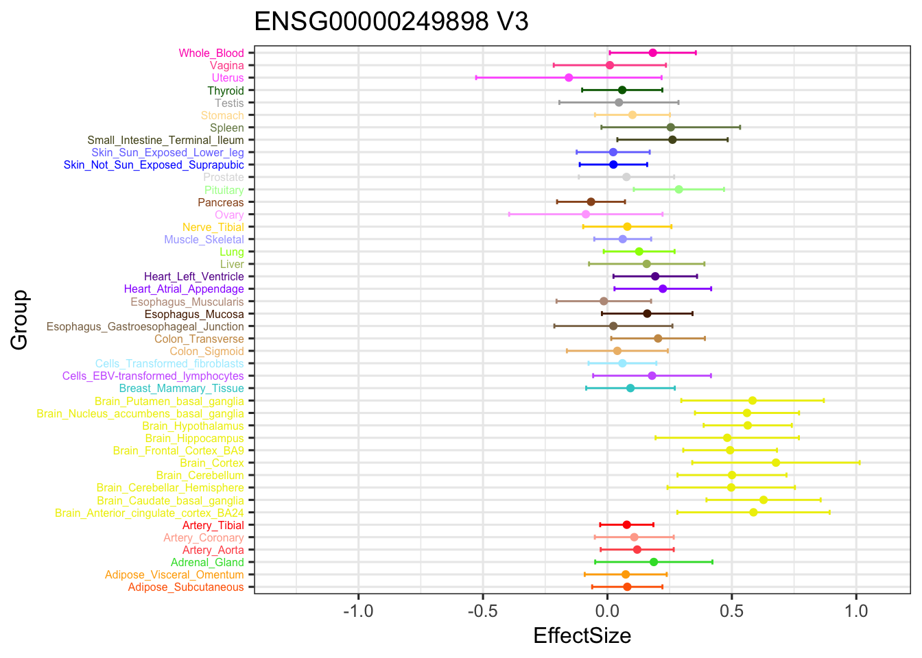

The gene significant in V3 EZ, not in current EZ:

ind = setdiff(get_significant_results(m_V3_EZ), get_significant_results(m_current_EZ))[1]
par(mfrow=c(1,3))

stronggene = data.frame(gtex$strong.b[ind,])
colnames(stronggene) = 'EffectSize'
stronggene$Group = row.names(stronggene)
stronggene$se = gtex$strong.s[ind,]
ggplot(stronggene, aes(y = EffectSize, x = Group)) + 
  geom_point(show.legend = FALSE, color=gtex.colors) + coord_flip() + ggtitle('ENSG00000126243') + ylim(c(-1.3,1.1)) + geom_errorbar(aes(ymin=EffectSize-1.96*se, ymax=EffectSize+1.96*se), width=0.4, show.legend = FALSE, color=gtex.colors) + 
  theme_bw(base_size=12) + theme(axis.text.y = element_text(colour = gtex.colors, size = 6))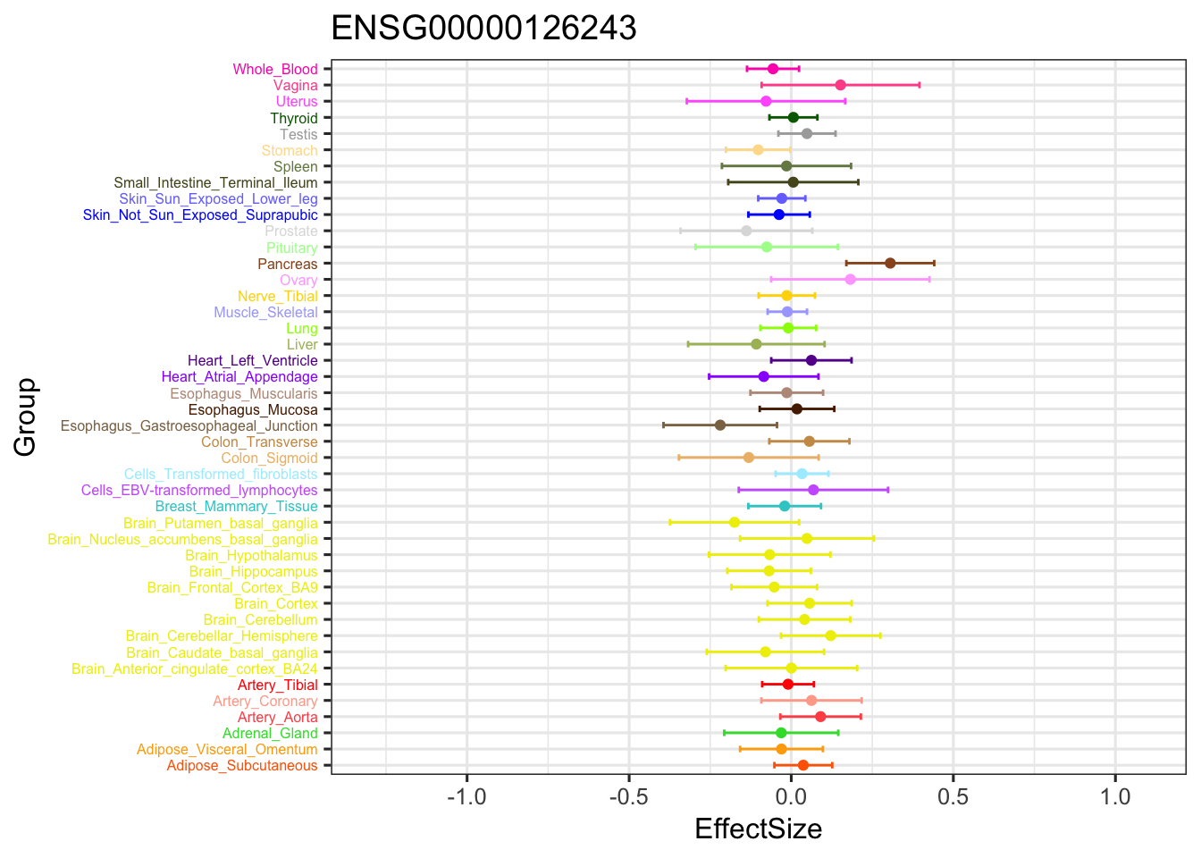

stronggeneCurrent = data.frame(m_current_EZ$result$PosteriorMean[ind,])
colnames(stronggeneCurrent) = 'EffectSize'
stronggeneCurrent$Group = row.names(stronggeneCurrent)
stronggeneCurrent$se = m_current_EZ$result$PosteriorSD[ind,]
ggplot(stronggeneCurrent, aes(y = EffectSize, x = Group)) + 
  geom_point(show.legend = FALSE, color=gtex.colors) + coord_flip() + ggtitle('ENSG00000126243 Current') + ylim(c(-1.3,1.1)) + 
  geom_errorbar(aes(ymin=EffectSize-1.96*se, ymax=EffectSize+1.96*se), width=0.4, show.legend = FALSE, color=gtex.colors) + 
  theme_bw(base_size=12) + theme(axis.text.y = element_text(colour = gtex.colors, size = 6))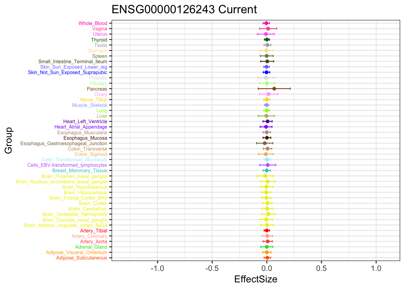

stronggeneV3 = data.frame(m_V3_EZ$result$PosteriorMean[ind,])
colnames(stronggeneV3) = 'EffectSize'
stronggeneV3$Group = row.names(stronggeneV3)
stronggeneV3$se = m_V3_EZ$result$PosteriorSD[ind,]
ggplot(stronggeneV3, aes(y = EffectSize, x = Group)) + 
  geom_point(show.legend = FALSE, color=gtex.colors) + ylim(c(-1.3,1.1)) + coord_flip() + ggtitle('ENSG00000126243 V3') + 
  geom_errorbar(aes(ymin=EffectSize-1.96*se, ymax=EffectSize+1.96*se), width=0.4, show.legend = FALSE, color=gtex.colors) + 
  theme_bw(base_size=12) + theme(axis.text.y = element_text(colour = gtex.colors, size = 6))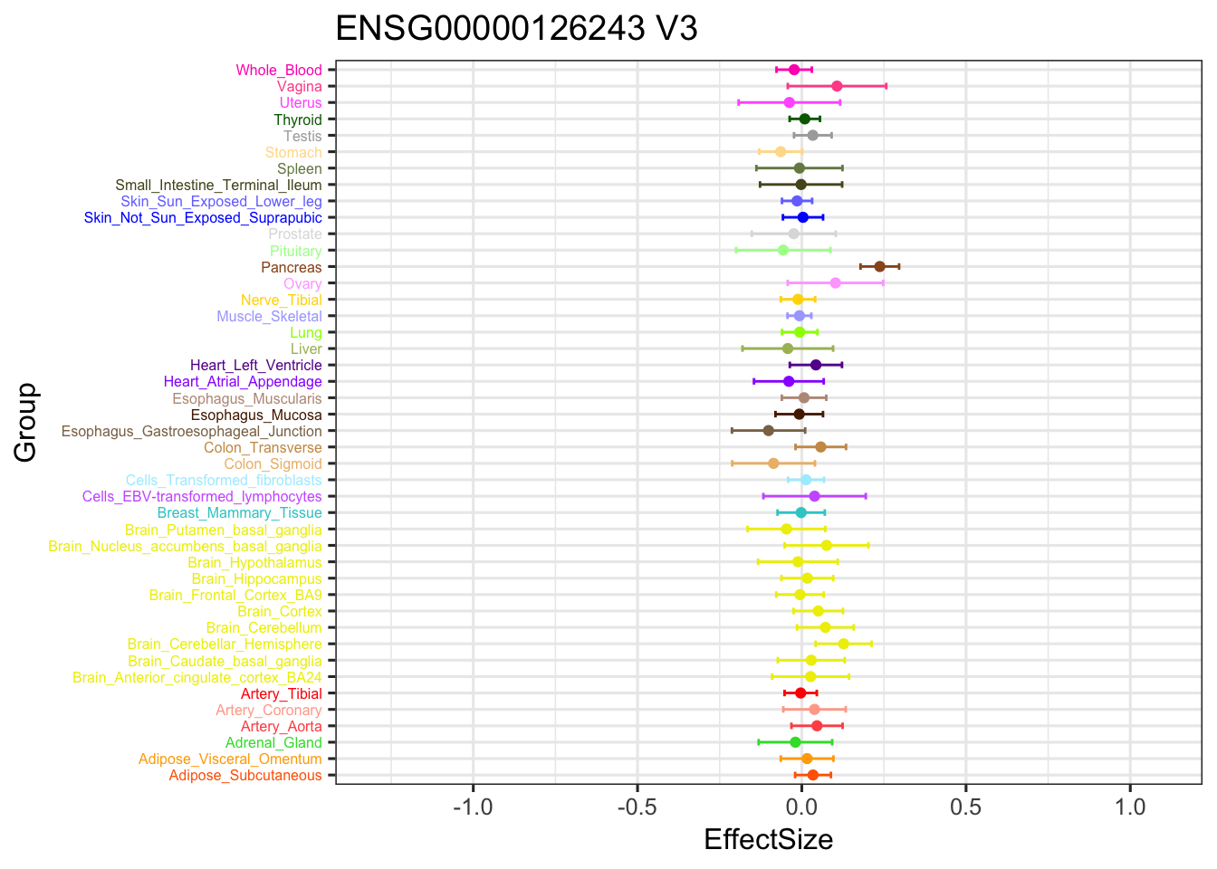

The pairwise sharing by magnitude

par(mfrow = c(1,2))
x           <- get_pairwise_sharing(m_ignore_EZ)
colnames(x) <- colnames(get_lfsr(m_ignore_EZ))
rownames(x) <- colnames(x)
clrs=colorRampPalette(rev(c('darkred', 'red','orange','yellow','cadetblue1', 'cyan', 'dodgerblue4', 'blue','darkorchid1','lightgreen','green', 'forestgreen','darkolivegreen')))(200)

corrplot::corrplot(x, method='color', type='upper', tl.col="black", tl.srt=45, tl.cex = 0.7, diag = FALSE, col=clrs, cl.lim = c(0,1), title = 'Ignore EZ', mar=c(0,0,5,0))

Warning in corrplot::corrplot(x, method = "color", type = "upper", tl.col =
"black", : Not been able to calculate text margin, please try again with a
clean new empty window using {plot.new(); dev.off()} or reduce tl.cex

x           <- get_pairwise_sharing(m_simple_EZ)
colnames(x) <- colnames(get_lfsr(m_simple_EZ))
rownames(x) <- colnames(x)

corrplot::corrplot(x, method='color', type='upper', tl.col="black", tl.srt=45, tl.cex = 0.7, diag = FALSE, col=clrs, cl.lim = c(0,1), title = 'Simple EZ', mar=c(0,0,5,0))

Warning in corrplot::corrplot(x, method = "color", type = "upper", tl.col =
"black", : Not been able to calculate text margin, please try again with a
clean new empty window using {plot.new(); dev.off()} or reduce tl.cex

par(mfrow=c(1,2))
x           <- get_pairwise_sharing(m_current_EZ)
colnames(x) <- colnames(get_lfsr(m_current_EZ))
rownames(x) <- colnames(x)
corrplot::corrplot(x, method='color', type='upper', tl.col="black", tl.srt=45, tl.cex = 0.7, diag = FALSE, col=clrs, cl.lim = c(0,1), title = 'Current EZ', mar=c(0,0,5,0))

Warning in corrplot::corrplot(x, method = "color", type = "upper", tl.col =
"black", : Not been able to calculate text margin, please try again with a
clean new empty window using {plot.new(); dev.off()} or reduce tl.cex

x           <- get_pairwise_sharing(m_V3_EZ)
colnames(x) <- colnames(get_lfsr(m_V3_EZ))
rownames(x) <- colnames(x)
corrplot::corrplot(x, method='color', type='upper', tl.col="black", tl.srt=45, tl.cex = 0.7, diag = FALSE, col=clrs, cl.lim = c(0,1), title = 'V3 EZ', mar=c(0,0,5,0))

Warning in corrplot::corrplot(x, method = "color", type = "upper", tl.col =
"black", : Not been able to calculate text margin, please try again with a
clean new empty window using {plot.new(); dev.off()} or reduce tl.cex

Session information

sessionInfo()

R version 3.5.1 (2018-07-02)
Platform: x86_64-apple-darwin15.6.0 (64-bit)
Running under: macOS  10.14.2

Matrix products: default
BLAS: /Library/Frameworks/R.framework/Versions/3.5/Resources/lib/libRblas.0.dylib
LAPACK: /Library/Frameworks/R.framework/Versions/3.5/Resources/lib/libRlapack.dylib

locale:
[1] en_US.UTF-8/en_US.UTF-8/en_US.UTF-8/C/en_US.UTF-8/en_US.UTF-8

attached base packages:
[1] stats     graphics  grDevices utils     datasets  methods   base     

other attached packages:
[1] ggplot2_3.1.0     kableExtra_0.9.0  knitr_1.20        mclust_5.4.1     
[5] mashr_0.2.19.0555 ashr_2.2-26       mixsqp_0.1-93     flashr_0.6-3     

loaded via a namespace (and not attached):
 [1] softImpute_1.4    tidyselect_0.2.5  corrplot_0.84    
 [4] purrr_0.2.5       reshape2_1.4.3    lattice_0.20-35  
 [7] colorspace_1.3-2  viridisLite_0.3.0 htmltools_0.3.6  
[10] yaml_2.2.0        rlang_0.3.0.1     R.oo_1.22.0      
[13] pillar_1.3.1      withr_2.1.2       glue_1.3.0       
[16] R.utils_2.7.0     bindrcpp_0.2.2    foreach_1.4.4    
[19] plyr_1.8.4        bindr_0.1.1       stringr_1.3.1    
[22] munsell_0.5.0     gtable_0.2.0      workflowr_1.1.1  
[25] rvest_0.3.2       R.methodsS3_1.7.1 mvtnorm_1.0-8    
[28] codetools_0.2-15  evaluate_0.12     labeling_0.3     
[31] pscl_1.5.2        doParallel_1.0.14 parallel_3.5.1   
[34] highr_0.7         Rcpp_1.0.0        readr_1.1.1      
[37] scales_1.0.0      backports_1.1.2   rmeta_3.0        
[40] truncnorm_1.0-8   abind_1.4-5       hms_0.4.2        
[43] digest_0.6.18     stringi_1.2.4     dplyr_0.7.6      
[46] grid_3.5.1        rprojroot_1.3-2   tools_3.5.1      
[49] magrittr_1.5      lazyeval_0.2.1    tibble_1.4.2     
[52] crayon_1.3.4      whisker_0.3-2     pkgconfig_2.0.2  
[55] MASS_7.3-50       Matrix_1.2-14     xml2_1.2.0       
[58] SQUAREM_2017.10-1 httr_1.3.1        rstudioapi_0.8   
[61] assertthat_0.2.0  rmarkdown_1.10    iterators_1.0.10 
[64] R6_2.3.0          git2r_0.23.0      compiler_3.5.1

This reproducible R Markdown analysis was created with workflowr 1.1.1

GTEx V6

Yuxin Zou

2018-12-20

Data Driven Covariances

Session information