Introduction
Here I again fit nonnegative loadings to the “strong” GTEx dataset, but I now use the trick discussed here to fit a non-diagonal error covariance matrix \(V\).
I pre-run the code below and load the results from file.
Comparison with previous results
Whereas my earlier analysis (which implicitly assumed that \(V = I\)) found 39 data-driven loadings, here I was only able to 26 obtain loadings.
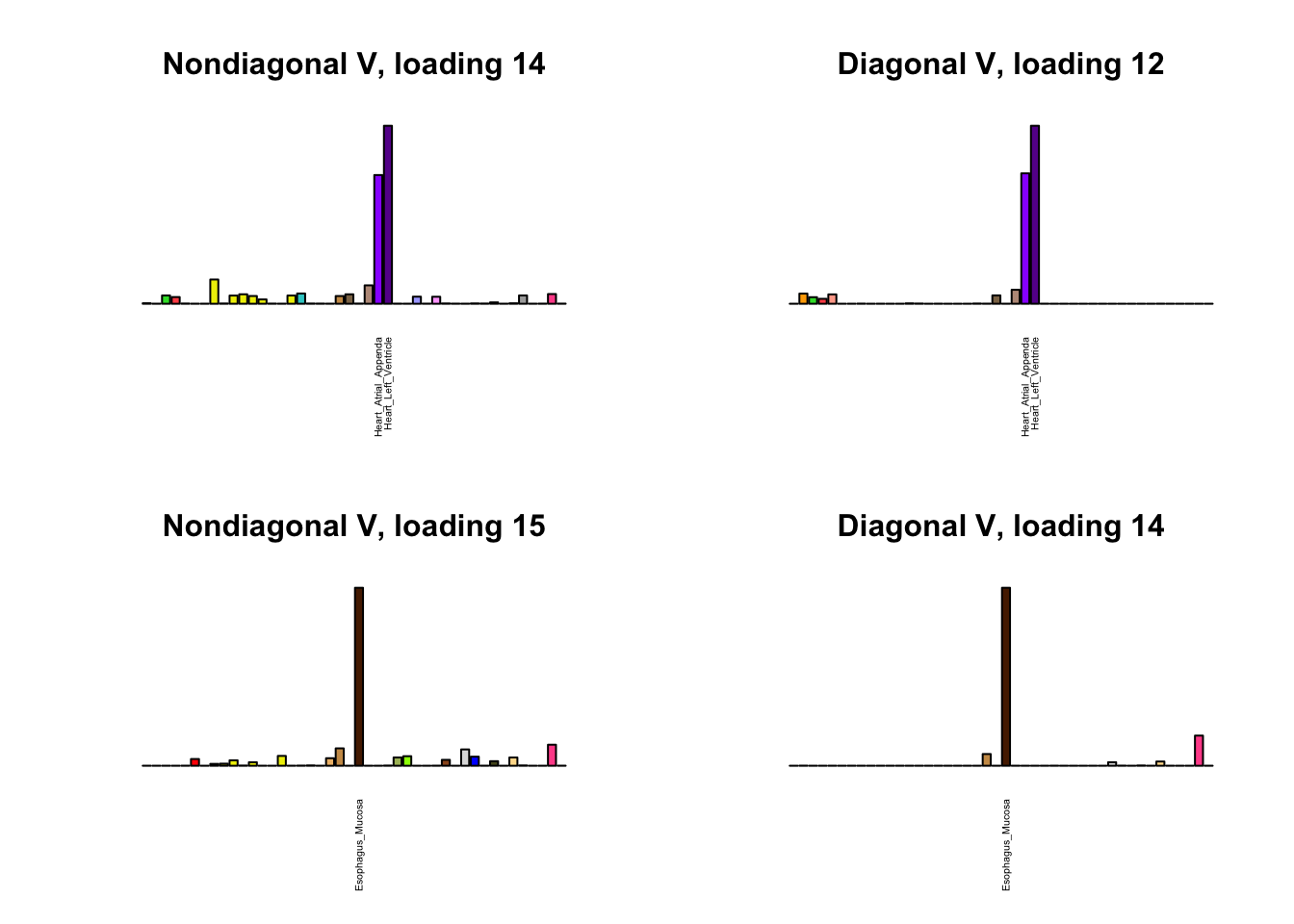
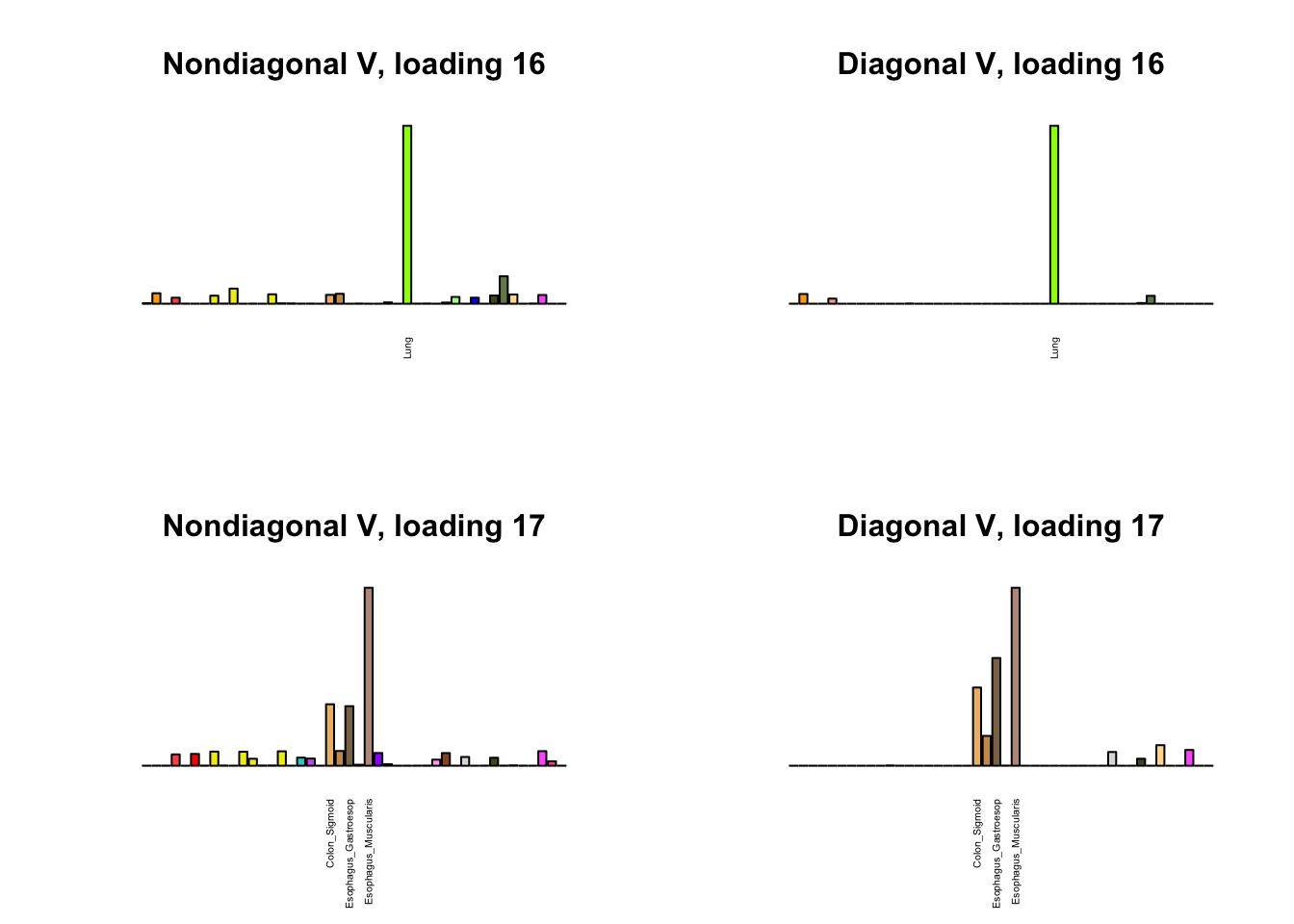
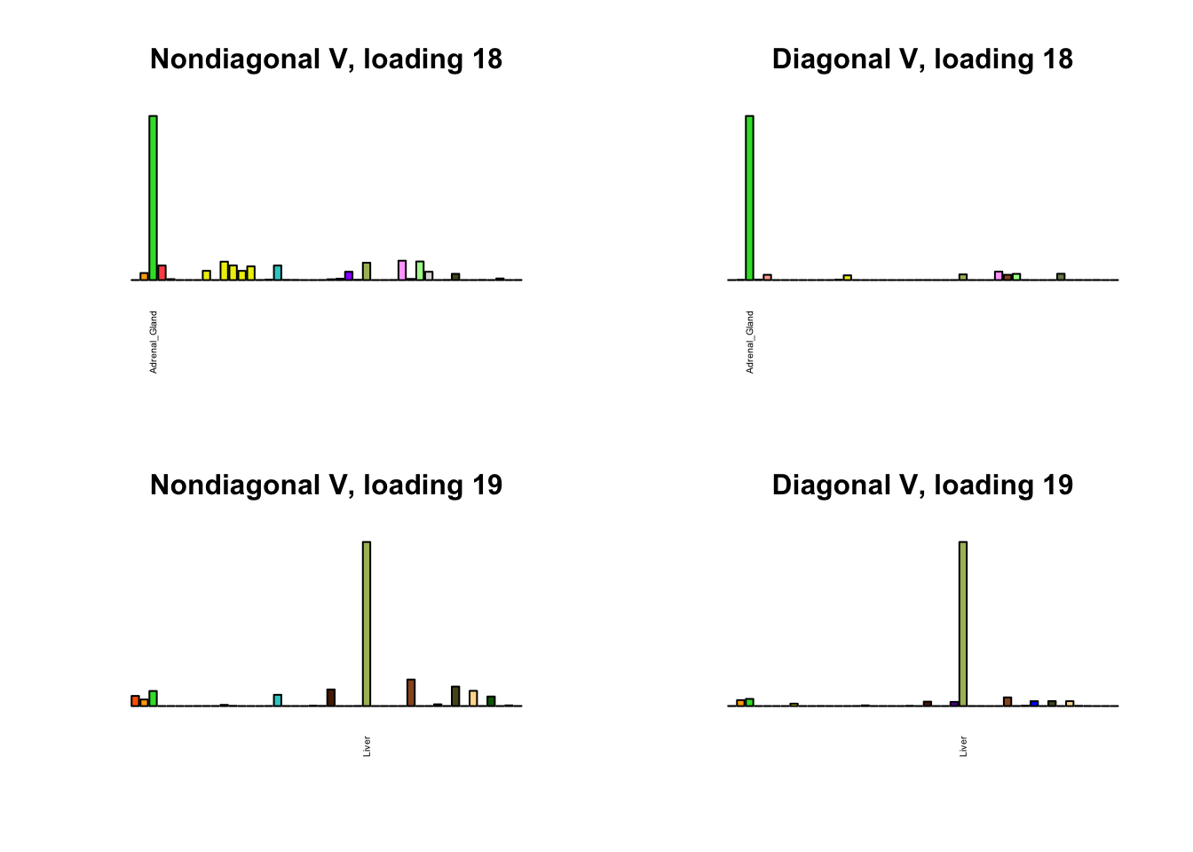
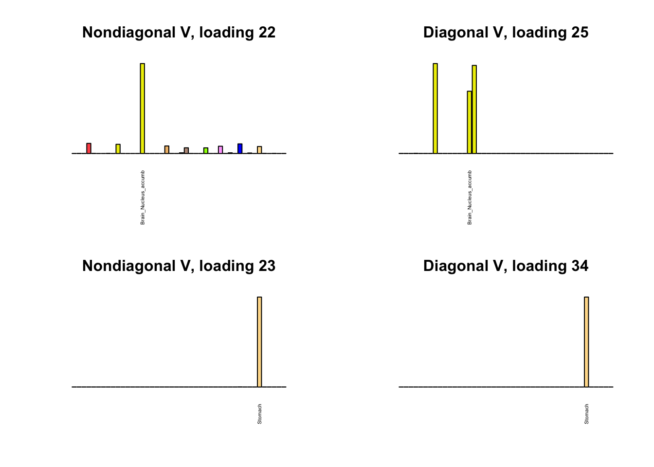
Similar loadings
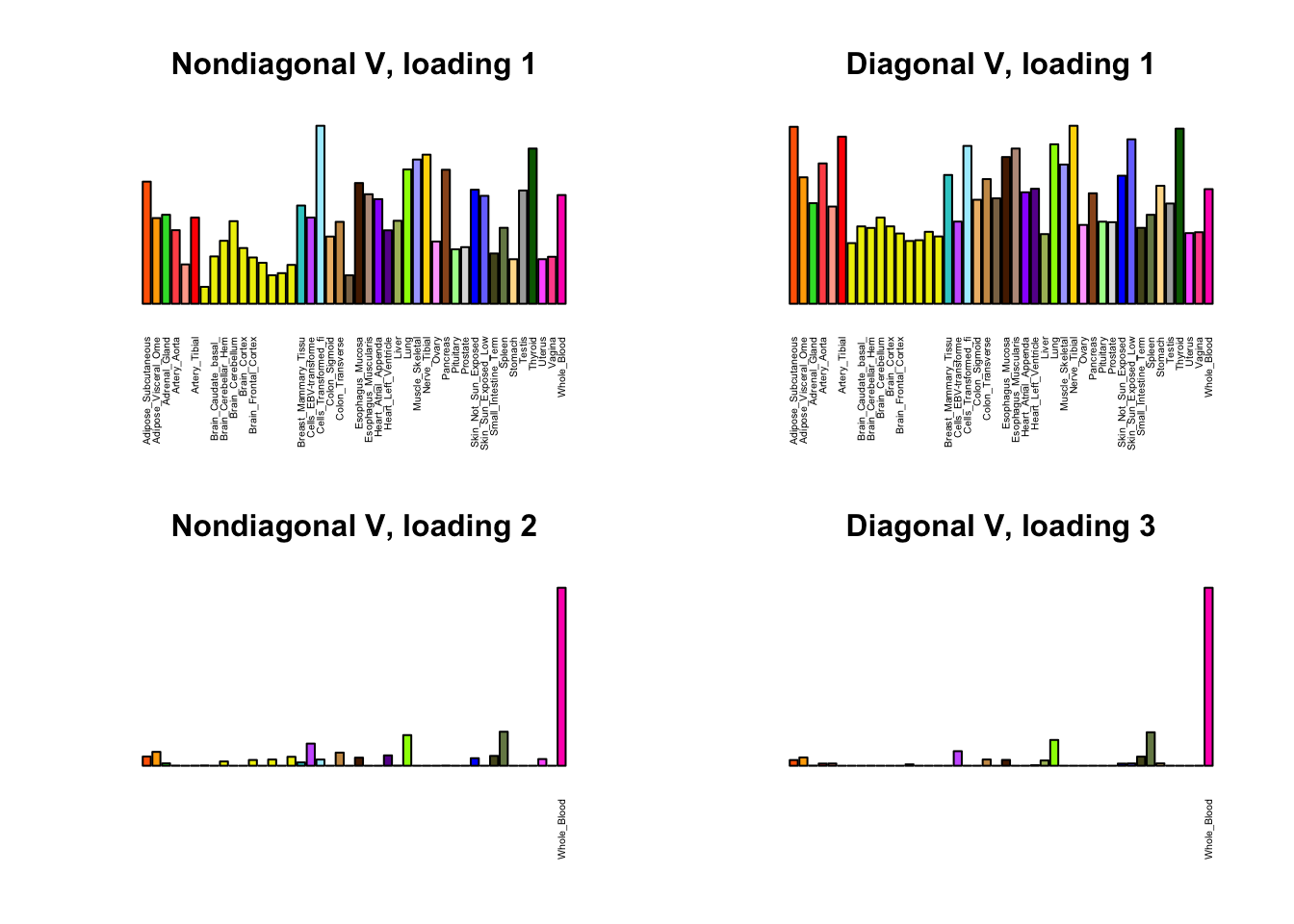
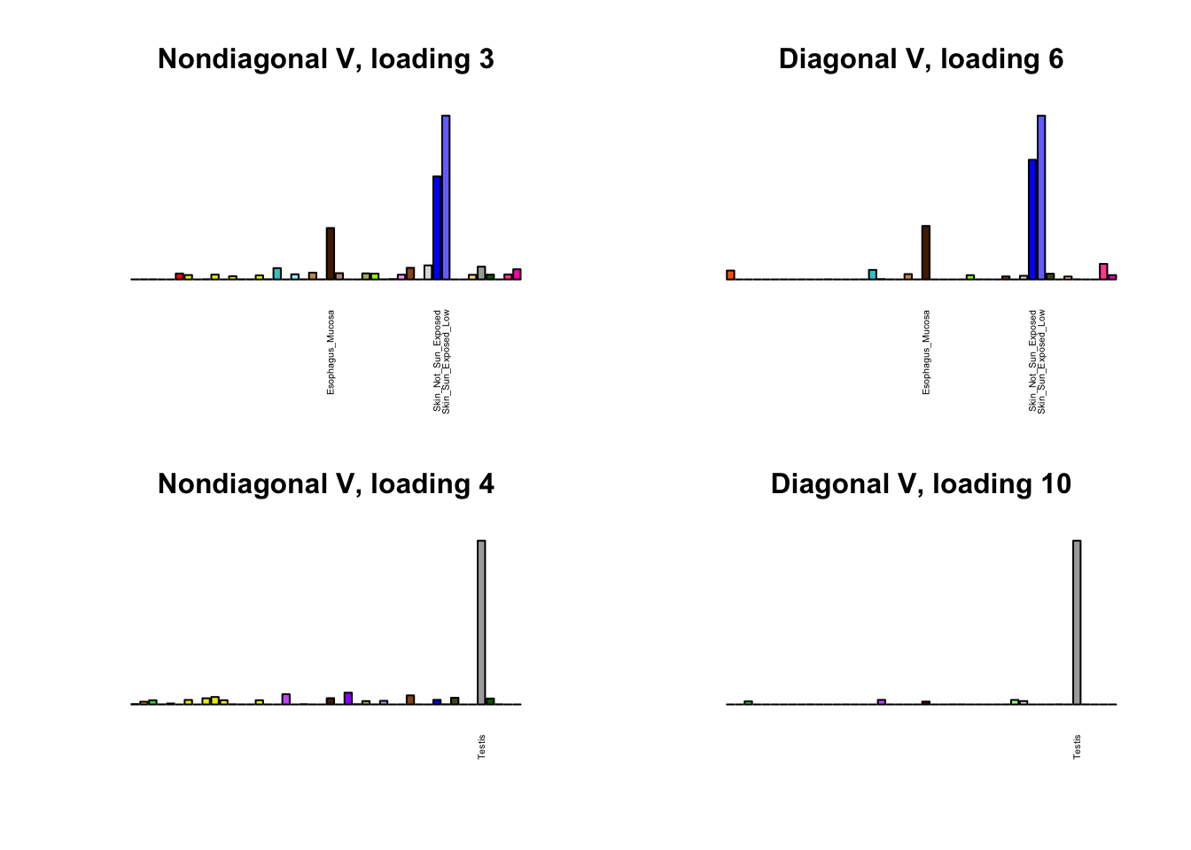
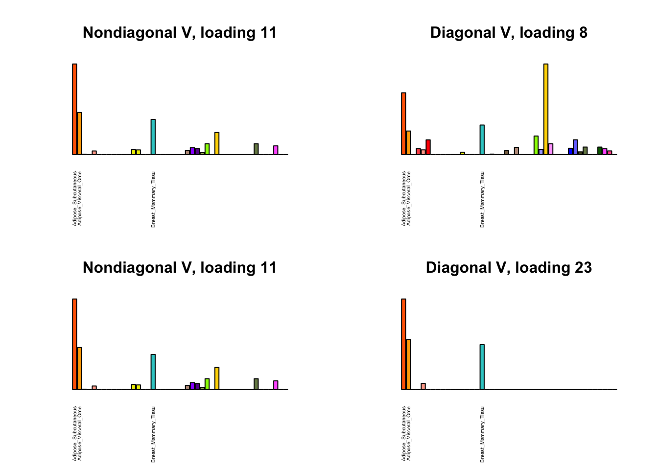
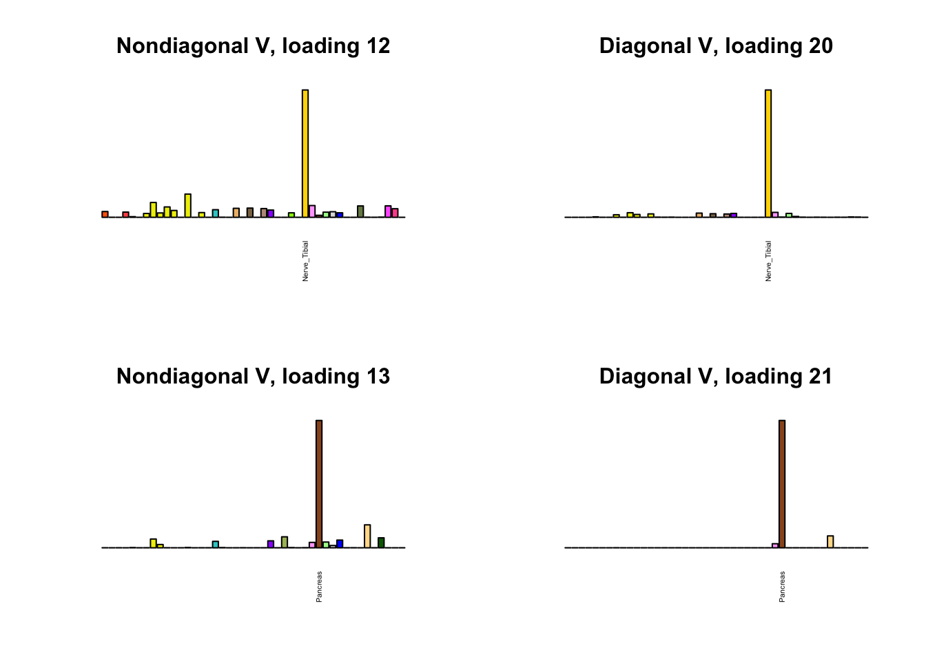
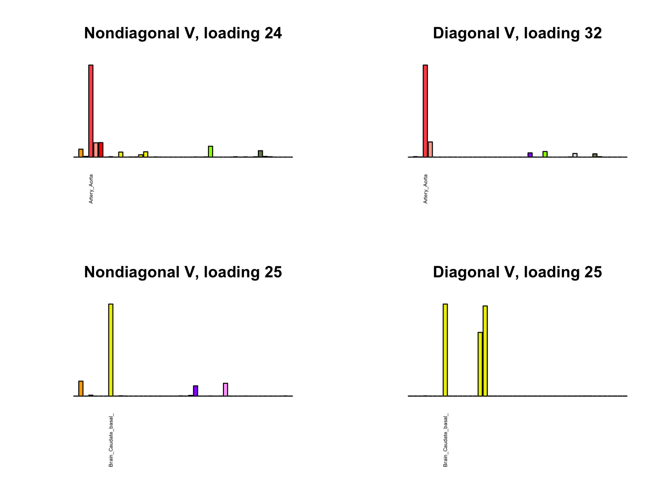
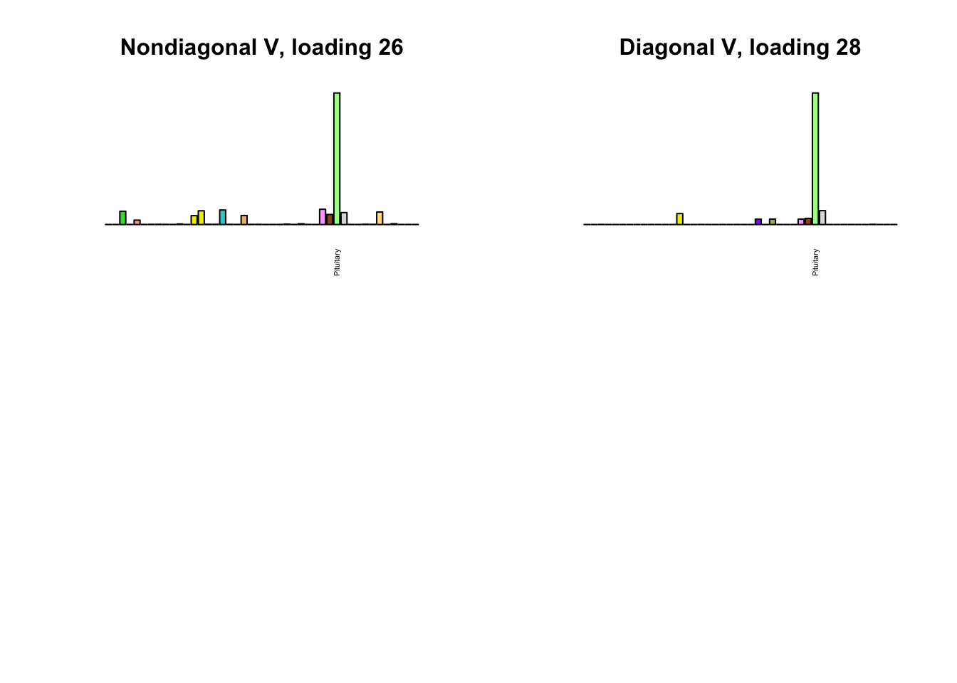
I first plot the new loadings side by side with the previous loadings to which they most closely correspond. Note that, in general, the previous loadings tend to be sparser than these new loadings. Further, this new approach finds two unique effects (caudate basal ganglia and nucleus accumbens basal ganglia) where the previous approach very plausibly found correlations among three types of basal ganglia (loading 25). However, the adipose tissue effects (loading 11) do not get tangled up with the tibial nerve tissue effect (as they did in the previous approach).
nondiag <- readRDS("./output/MASHvFLASHnondiagonalV/2dRepeat3.rds")
diag <- readRDS("./output/MASHvFLASHnn/fl.rds")

nondiag_order <- c(44:54, 54:nondiag$nfactors)
diag_order <- c(1, 3, 6, 10,
                4, 9, 7, 15,
                5, 13, 8, 23, 20,
                21, 12, 14, 16,
                17, 18, 19, 2,
                24, 25, 34, 32,
                25, 28)

diag_not_nondiag <- setdiff(c(1:29, 31:40), diag_order)

tissue_names <- rownames(diag$EL)

missing.tissues <- c(7, 8, 19, 20, 24, 25, 31, 34, 37)
gtex.colors <- read.table("https://github.com/stephenslab/gtexresults/blob/master/data/GTExColors.txt?raw=TRUE", sep = '\t', comment.char = '')[-missing.tissues, 2]
gtex.colors <- as.character(gtex.colors)

par(mfrow=c(2,2))
display_names <- strtrim(tissue_names, 20)
for(i in 1:length(nondiag_order)) {
  plot_names <- display_names

  next_nondiag <- nondiag$fit$EL[, nondiag_order[i]]
  plot_names[next_nondiag < 0.25 * max(next_nondiag)] <- ""
  barplot(next_nondiag,
          main=paste0('Nondiagonal V, loading ', nondiag_order[i] - 43),
          las=2, cex.names=0.4, yaxt='n',
          col=gtex.colors, names=plot_names)

  barplot(diag$EL[, diag_order[i]],
          main=paste0('Diagonal V, loading ', diag_order[i]),
          las=2, cex.names=0.4, yaxt='n',
          col=gtex.colors, names=plot_names)
}


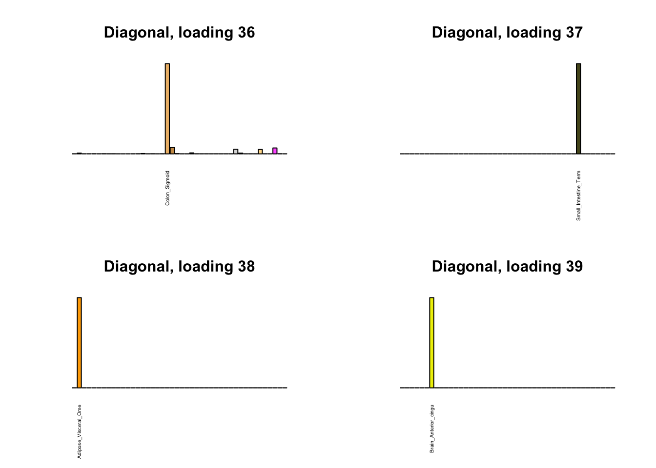
Differences
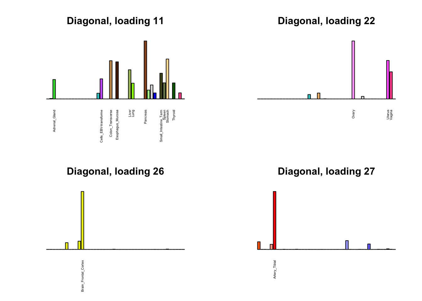
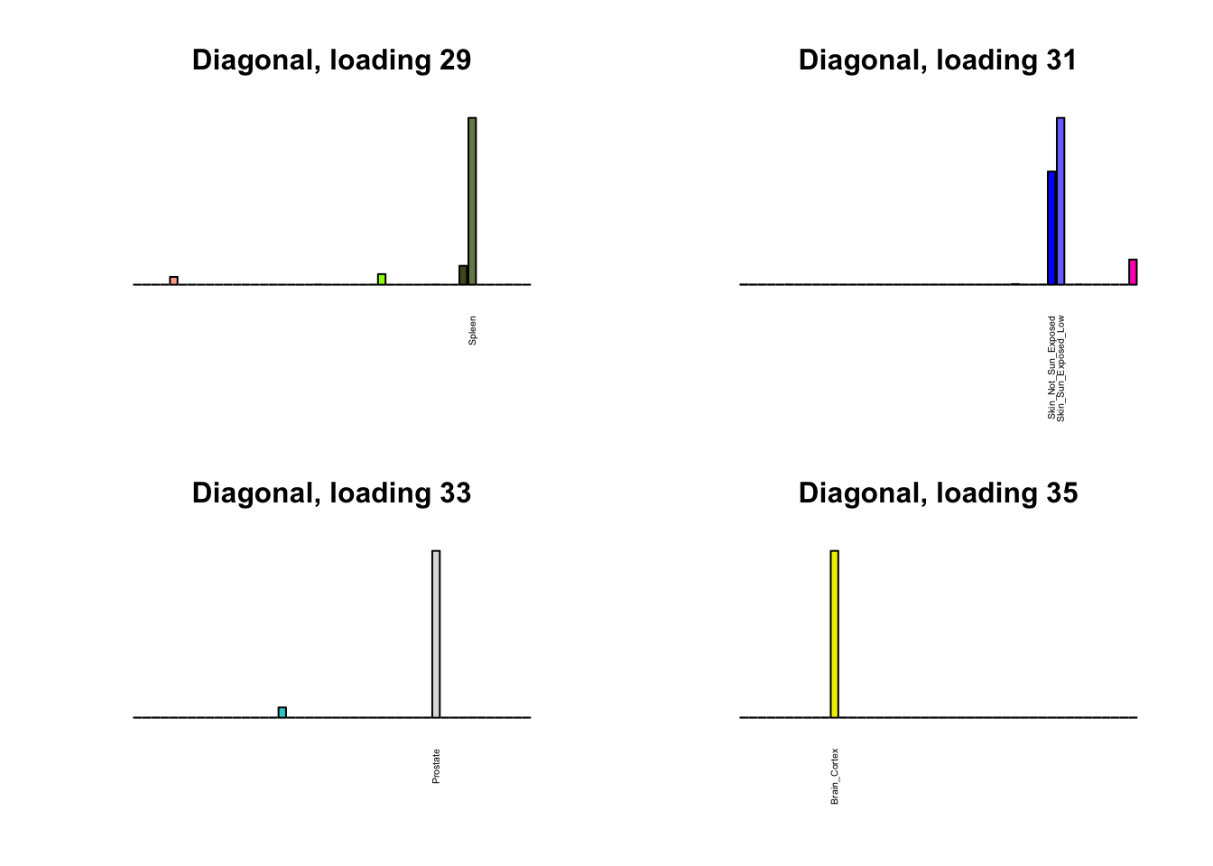
Next, I plot previous loadings that do not correspond to any of the new loadings. One of these (loading 11) may indeed be an artefactual loading that corresponds to covariance in errors rather than biological reality. However, two of the others (loadings 22 and 31) describe very plausible correlations (among ovarian, uterine, and vaginal tissues on the one hand, and among sun-exposed and non-exposed skin tissues on the other). The remaining are unique effects.
par(mfrow=c(2,2))
for (i in 1:length(diag_not_nondiag)) {
  plot_names <- display_names

  next_diag <- diag$EL[, diag_not_nondiag[i]]
  plot_names[next_diag < 0.25 * max(next_diag)] <- ""
  barplot(next_diag,
          main=paste0('Diagonal, loading ', diag_not_nondiag[i]),
          las=2, cex.names=0.4, yaxt='n',
          col=gtex.colors, names=plot_names)
}

Code
Click “Code” to view the code used to obtain the above results.
devtools::load_all("/Users/willwerscheid/GitHub/flashr/")
devtools::load_all("/Users/willwerscheid/GitHub/ebnm/")

library(mashr)

gtex <- readRDS(gzcon(url("https://github.com/stephenslab/gtexresults/blob/master/data/MatrixEQTLSumStats.Portable.Z.rds?raw=TRUE")))

strong <- gtex$strong.z
random <- gtex$random.z

# Step 1. Estimate correlation structure using MASH.

m_random <- mash_set_data(random, Shat = 1)
Vhat <- estimate_null_correlation(m_random)

# Step 2. Estimate data-driven loadings using FLASH.

# Step 2a. Fit Vhat.
n <- nrow(Vhat)
lambda.min <- min(eigen(Vhat, symmetric=TRUE, only.values=TRUE)$values)

data <- flash_set_data(Y, S = sqrt(lambda.min))

W.eigen <- eigen(Vhat - diag(rep(lambda.min, n)), symmetric=TRUE)
# The rank of W is at most n - 1, so we can drop the last eigenval/vec:
W.eigen$values <- W.eigen$values[-n]
W.eigen$vectors <- W.eigen$vectors[, -n, drop=FALSE]

fl <- flash_add_fixed_loadings(data,
                               LL=W.eigen$vectors,
                               init_fn="udv_svd",
                               backfit=FALSE)

ebnm_param_f <- lapply(as.list(W.eigen$values),
                       function(eigenval) {
                         list(g = list(a=1/eigenval, pi0=0), fixg = TRUE)
                       })
ebnm_param_l <- lapply(vector("list", n - 1),
                       function(k) {list()})
fl <- flash_backfit(data,
                    fl,
                    var_type="zero",
                    ebnm_fn="ebnm_pn",
                    ebnm_param=(list(f = ebnm_param_f, l = ebnm_param_l)),
                    nullcheck=FALSE)

# Step 2b. Add nonnegative factors.
ebnm_fn = list(f = "ebnm_pn", l = "ebnm_ash")
ebnm_param = list(f = list(warmstart = TRUE),
                  l = list(mixcompdist="+uniform"))
fl <- flash_add_greedy(data,
                       Kmax=50,
                       f_init=fl,
                       var_type="zero",
                       init_fn="udv_svd",
                       ebnm_fn=ebnm_fn,
                       ebnm_param=ebnm_param)
saveRDS(fl, "./output/MASHvFLASHVhat/2bGreedy.rds")

# Step 2c (optional). Backfit factors from step 2b.
fl <- flash_backfit(data,
                    fl,
                    kset=n:fl$nfactors,
                    var_type="zero",
                    ebnm_fn=ebnm_fn,
                    ebnm_param=ebnm_param,
                    nullcheck=FALSE)
saveRDS(fl, "./output/MASHvFLASHVhat/2cBackfit.rds")

# Step 2d (optional). Repeat steps 2b and 2c as desired.
fl <- flash_add_greedy(data,
                       Kmax=50,
                       f_init=fl,
                       var_type="zero",
                       init_fn="udv_svd",
                       ebnm_fn=ebnm_fn,
                       ebnm_param=ebnm_param)
fl <- flash_backfit(data,
                    fl,
                    kset=n:fl$nfactors,
                    var_type="zero",
                    ebnm_fn=ebnm_fn,
                    ebnm_param=ebnm_param,
                    nullcheck=FALSE)
saveRDS(fl, "./output/MASHvFLASHVhat/2dRepeat3.rds")
Session information
sessionInfo()R version 3.4.3 (2017-11-30)
Platform: x86_64-apple-darwin15.6.0 (64-bit)
Running under: macOS High Sierra 10.13.6
Matrix products: default
BLAS: /Library/Frameworks/R.framework/Versions/3.4/Resources/lib/libRblas.0.dylib
LAPACK: /Library/Frameworks/R.framework/Versions/3.4/Resources/lib/libRlapack.dylib
locale:
[1] en_US.UTF-8/en_US.UTF-8/en_US.UTF-8/C/en_US.UTF-8/en_US.UTF-8
attached base packages:
[1] stats graphics grDevices utils datasets methods base
loaded via a namespace (and not attached):
[1] workflowr_1.0.1 Rcpp_0.12.17 digest_0.6.15
[4] rprojroot_1.3-2 R.methodsS3_1.7.1 backports_1.1.2
[7] git2r_0.21.0 magrittr_1.5 evaluate_0.10.1
[10] stringi_1.1.6 whisker_0.3-2 R.oo_1.21.0
[13] R.utils_2.6.0 rmarkdown_1.8 tools_3.4.3
[16] stringr_1.3.0 yaml_2.1.17 compiler_3.4.3
[19] htmltools_0.3.6 knitr_1.20 This reproducible R Markdown analysis was created with workflowr 1.0.1