Matrix factorization of count data
Jason Willwerscheid
9/20/2018
Last updated: 2018-09-21
workflowr checks: (Click a bullet for more information)-
✔ R Markdown file: up-to-date
Great! Since the R Markdown file has been committed to the Git repository, you know the exact version of the code that produced these results.
-
✔ Environment: empty
Great job! The global environment was empty. Objects defined in the global environment can affect the analysis in your R Markdown file in unknown ways. For reproduciblity it’s best to always run the code in an empty environment.
-
✔ Seed:
set.seed(20180714)The command
set.seed(20180714)was run prior to running the code in the R Markdown file. Setting a seed ensures that any results that rely on randomness, e.g. subsampling or permutations, are reproducible. -
✔ Session information: recorded
Great job! Recording the operating system, R version, and package versions is critical for reproducibility.
-
Great! You are using Git for version control. Tracking code development and connecting the code version to the results is critical for reproducibility. The version displayed above was the version of the Git repository at the time these results were generated.✔ Repository version: 884f8fa
Note that you need to be careful to ensure that all relevant files for the analysis have been committed to Git prior to generating the results (you can usewflow_publishorwflow_git_commit). workflowr only checks the R Markdown file, but you know if there are other scripts or data files that it depends on. Below is the status of the Git repository when the results were generated:
Note that any generated files, e.g. HTML, png, CSS, etc., are not included in this status report because it is ok for generated content to have uncommitted changes.Ignored files: Ignored: .DS_Store Ignored: .Rhistory Ignored: .Rproj.user/ Ignored: docs/.DS_Store Ignored: docs/figure/.DS_Store Untracked files: Untracked: code/pois_lik.R Untracked: data/greedy19.rds Untracked: temp_debug.RDS
Expand here to see past versions:
| File | Version | Author | Date | Message |
|---|---|---|---|---|
| Rmd | 884f8fa | Jason Willwerscheid | 2018-09-21 | wflow_publish(“analysis/count_data.Rmd”) |
Introduction
In a previous analysis, I used FLASH to obtain a nonnegative matrix factorization of the GTEx donation matrix. There, I proceeded as if the observations were normally distributed. Here, I explore a more sophisticated approach to count data.
Model
I assume that the data is generated as \[ Y \sim \text{Poisson}(\mu), \] where \[ \mu = LF' = \sum_{k = 1}^K l_k f_k', \] with an ASH prior on the entries of each loading \(l_k\) and each factor \(f_k\) \[ l_k \sim g_{l_k},\ f_k \sim g_{f_k}. \]
Idea
The general idea is outlined by Matthew Stephens here.
To apply the idea to FLASH, I replace the part of the objective function that comes from the residuals with the Poisson log likelihood \[ \ell(\mu) = \sum_{i, j} -\mu_{ij} + Y_{ij} \log \mu_{ij}. \] Set \(\eta_{ij} = \log \mu_{ij}\) so that \[ \ell(\eta) = \sum_{i, j} -e^{\eta_{ij}} + Y_{ij} \eta_{ij}. \]
Now do a second-order Taylor expansion of \(\ell(\eta)\) around some (for now, arbitrary) point \(\eta^\star\): \[ \ell(\eta) = \ell(\eta^\star) + (\eta - \eta^\star) \ell'(\eta^\star) + \frac{(\eta - \eta^\star)^2}{2} \ell''(\eta^\star). \]
This is precisely the log likelihood for the distribution \[ \eta \sim \text{Normal}\left(\eta^\star - \frac{\ell''(\eta^\star)}{\ell'(\eta^\star)}, -\frac{1}{\ell''(\eta^\star)}\right). \]
Thus, given a good enough choice of \(\eta^\star\), we should be able to run FLASH on the “pseudo-data” \[ X = \eta^\star - \frac{\ell''(\eta^\star)}{\ell'(\eta^\star)} = \log(\mu^\star) + \frac{Y - \mu^\star}{\mu^\star}\] with “standard errors” \[S = -\frac{1}{\sqrt{\ell''(\mu^\star)}} = \frac{1}{\sqrt{\mu^\star}}, \] where \(\mu^\star = e^{\eta^\star}\).
The crux, of course, is in choosing an \(\eta^\star\) that is close enough to the \(\eta\) that minimizes the objective function. An iterative procedure suggests itself whereby one fits FLASH to the pseudo-data generated by a given choice of \(\eta^\star\), then updates \(\eta^\star\) to be the posterior mean given by the FLASH fit, then fits FLASH to the pseudo-data generated by the new \(\eta^\star\), and so on until convergence.
Code and example
First I load the data:
devtools::load_all("~/GitHub/flashr")
#> Loading flashr
devtools::load_all("~/GitHub/ebnm")
#> Loading ebnm

raw <- read.csv("https://storage.googleapis.com/gtex_analysis_v6/annotations/GTEx_Data_V6_Annotations_SampleAttributesDS.txt",
                header=TRUE, sep='\t')

data <- raw[, c("SAMPID", "SMTSD")] # sample ID, tissue type
# Extract donor ID:
tmp <- strsplit(as.character(data$SAMPID), "-")
data$SAMPID <- as.factor(sapply(tmp, function(x) {x[[2]]}))
names(data) <- c("DonorID", "TissueType")

data <- suppressMessages(reshape2::acast(data, TissueType ~ DonorID))

missing.tissues <- c(1, 8, 9, 20, 21, 24, 26, 27, 33, 36, 39)
data <- data[-missing.tissues, ]

# Drop columns with no samples:
data = data[, colSums(data) > 0]

gtex.colors <- read.table("https://github.com/stephenslab/gtexresults/blob/master/data/GTExColors.txt?raw=TRUE",
                          sep = '\t', comment.char = '')
gtex.colors <- gtex.colors[-c(7, 8, 19, 20, 24, 25, 31, 34, 37), 2]
gtex.colors <- as.character(gtex.colors)
I will use the following functions to fit the model:
# Computing Poisson likelihood and FLASH ELBO --------------------------

pois_lik <- function(the_data, fl) {
  return(sum(-exp(fl$fitted_values) + the_data * fl$fitted_values))
}

pois_obj <- function(the_data, fl) {
  return(pois_lik(the_data, fl) + sum(unlist(fl$fit$KL_l)) +
           sum(unlist(fl$fit$KL_f)))
}

# Calculating pseudo-data ----------------------------------------------

calc_X <- function(the_data, mu) {
  return(log(mu) + (the_data - mu) / mu)
}

calc_S <- function(the_data, mu) {
  return(1 / sqrt(mu))
}

set_pseudodata <- function(the_data, mu) {
  return(flash_set_data(calc_X(the_data, mu), S = calc_S(the_data, mu)))
}

# Setting FLASH parameters ---------------------------------------------

# Initialization function for nonnegative loadings
#   (but arbitrary factors):
my_init_fn <- function(Y, K = 1) {
  ret = udv_svd(Y, K)
  n_pos = sum(ret$u > 0)
  n_neg = sum(ret$u < 0)
  if (n_neg > n_pos) {
    return(list(u = -ret$u, d = ret$d, v = -ret$v))
  } else
    return(ret)
}

get_init_fn <- function(nonnegative = FALSE) {
  if (nonnegative) {
    return("my_init_fn")
  } else {
    return("udv_svd")
  }
}

get_ebnm_fn <- function(nonnegative = FALSE) {
  if (nonnegative) {
    return(list(l = "ebnm_ash", f = "ebnm_pn"))
  } else {
    return(list(l = "ebnm_pn", f = "ebnm_pn"))
  }
}

get_ebnm_param <- function(nonnegative = FALSE) {
  if (nonnegative) {
    return(list(l = list(mixcompdist = "+uniform"),
                f = list(warmstart = TRUE)))
  } else {
    return(list(l = list(warmstart = TRUE),
                f = list(warmstart = TRUE)))
  }
}

# Initializing mu and running FLASH ------------------------------------

init_mu <- function(the_data, f_init) {
  if (is.null(f_init)) {
    return(matrix(colMeans(the_data),
                  nrow = nrow(the_data), ncol = ncol(the_data),
                  byrow = TRUE))
  } else {
    return(exp(f_init$fitted_values))
  }
}

greedy_iter <- function(the_data, mu, f_init, niter,
                        nonnegative = FALSE) {
  suppressWarnings(
    flash_greedy_workhorse(set_pseudodata(the_data, mu),
                           Kmax = 1,
                           f_init = f_init,
                           var_type = "zero",
                           ebnm_fn = get_ebnm_fn(nonnegative),
                           ebnm_param = get_ebnm_param(nonnegative),
                           init_fn = get_init_fn(nonnegative),
                           verbose_output = "",
                           nullcheck = FALSE,
                           maxiter = niter)
  )
}

backfit_iter <- function(the_data, mu, f_init, kset, niter,
                         nonnegative = FALSE) {
  suppressWarnings(
    flash_backfit_workhorse(set_pseudodata(the_data, mu),
                            kset = kset,
                            f_init = f_init,
                            var_type = "zero",
                            ebnm_fn = get_ebnm_fn(nonnegative),
                            ebnm_param = get_ebnm_param(nonnegative),
                            verbose_output = "",
                            nullcheck = FALSE,
                            maxiter = niter)
  )
}

run_one_fit <- function(the_data, f_init, greedy, maxiter = 200,
                        n_subiter = 200, nonnegative = FALSE,
                        verbose = TRUE, tol = .01) {
  mu <- init_mu(the_data, f_init)

  if (greedy) {
    fl <- greedy_iter(the_data, mu, f_init, n_subiter, nonnegative)
    kset <- ncol(fl$fit$EL) # Only "backfit" the greedily added factor
    mu <- exp(fl$fitted_values)
  } else {
    fl <- f_init
    kset <- 1:ncol(fl$fit$EL) # Backfit all factor/loadings
  }

  # The objective can get stuck oscillating between two values, so we
  #   need to track the last two values attained:
  old_old_obj <- -Inf
  old_obj <- -Inf
  diff <- Inf
  iter <- 0
  while (diff > tol && iter < maxiter) {
    iter <- iter + 1
    fl <- backfit_iter(the_data, mu, fl, kset, n_subiter, nonnegative)
    mu <- exp(fl$fitted_values)

    new_obj <- pois_obj(the_data, fl)
    diff <- min(abs(new_obj - old_obj), abs(new_obj - old_old_obj))

    old_old_obj <- old_obj
    old_obj <- new_obj

    if (verbose) {
      message("Iteration ", iter, ": ", old_obj)
    }
  }
  return(fl)
}
I greedily add a factor by initializing \(\mu^\star\) to the column means of the data, then alternating between running FLASH on the “pseudo-data” corresponding to the current \(\mu^\star\) and updating \(\mu^\star\) to be the posterior mean of the current FLASH fit:
fl <- run_one_fit(data, f_init = NULL, greedy = TRUE)
#> Iteration 1: -927714082346.181
#> Iteration 2: -341286945918.445
#> Iteration 3: -125552459516.84
#> Iteration 4: -46188177871.3924
#> Iteration 5: -16991690774.7395
#> Iteration 6: -6250903760.78647
#> Iteration 7: -2299589270.42295
#> Iteration 8: -845982056.385945
#> Iteration 9: -311229940.405073
#> Iteration 10: -114505696.365842
#> Iteration 11: -42134944.2935817
#> Iteration 12: -15511272.9754123
#> Iteration 13: -5717001.94860467
#> Iteration 14: -2113906.45466518
#> Iteration 15: -788404.890125627
#> Iteration 16: -300778.640349495
#> Iteration 17: -121382.535730719
#> Iteration 18: -55374.158506545
#> Iteration 19: -31079.0542736632
#> Iteration 20: -22130.6357421538
#> Iteration 21: -18834.2241948271
#> Iteration 22: -17631.9197964083
#> Iteration 23: -17227.1683461842
#> Iteration 24: -17120.3909758248
#> Iteration 25: -17094.2647075556
#> Iteration 26: -17091.0177410941
#> Iteration 27: -17090.5831181879
#> Iteration 28: -17090.5851822656
So, although the initial estimate of \(\mu^\star\) is terrible, the objective seems to eventually converge.
I continue to greedily add factors in the same way:
fl <- run_one_fit(data, f_init = fl, greedy = TRUE)
#> Iteration 1: -16012.4385475068
#> Iteration 2: -15996.0987462569
#> Iteration 3: -15994.474709406
#> Iteration 4: -15994.5035110124
#> Iteration 5: -15994.522807295
#> Iteration 6: -15994.5304893364
fl <- run_one_fit(data, f_init = fl, greedy = TRUE)
#> Iteration 1: -15994.5335404488
#> Iteration 2: -15994.5347437438
Since the third factor no longer offers any improvement, I stop adding factors and backfit:
fl <- run_one_fit(data, f_init = fl, greedy = FALSE)
#> Iteration 1: -15820.0913699191
#> Iteration 2: -15644.1196467394
#> Iteration 3: -15574.356156741
#> Iteration 4: -15526.9227894188
#> Iteration 5: -15503.4303568297
#> Iteration 6: -15492.9576959489
#> Iteration 7: -15488.9547268523
#> Iteration 8: -15487.6157343197
#> Iteration 9: -15487.1185250066
#> Iteration 10: -15486.8695270274
#> Iteration 11: -15486.7522169866
#> Iteration 12: -15486.7015595336
#> Iteration 13: -15486.6810231773
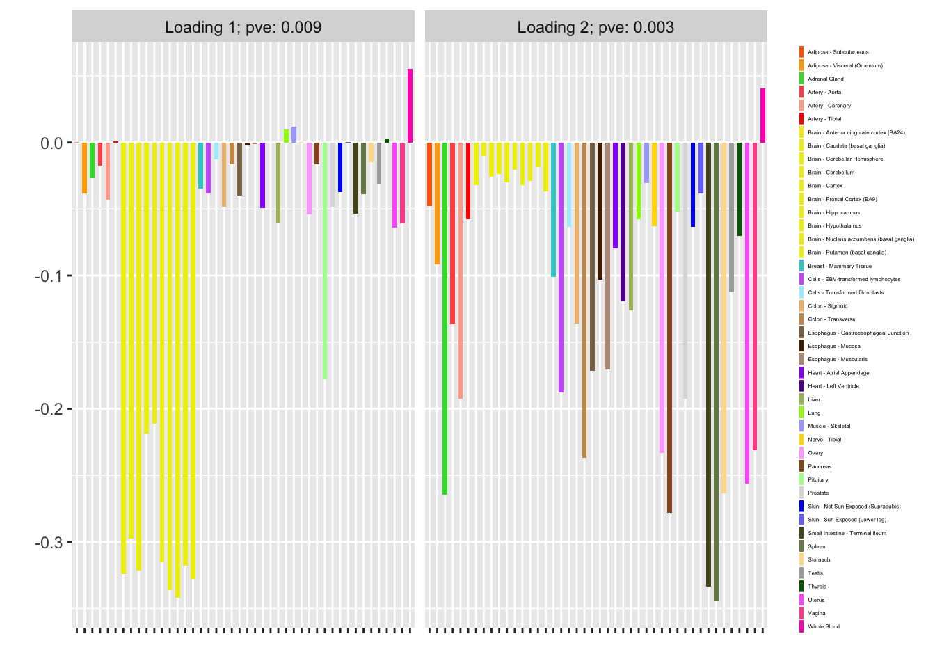
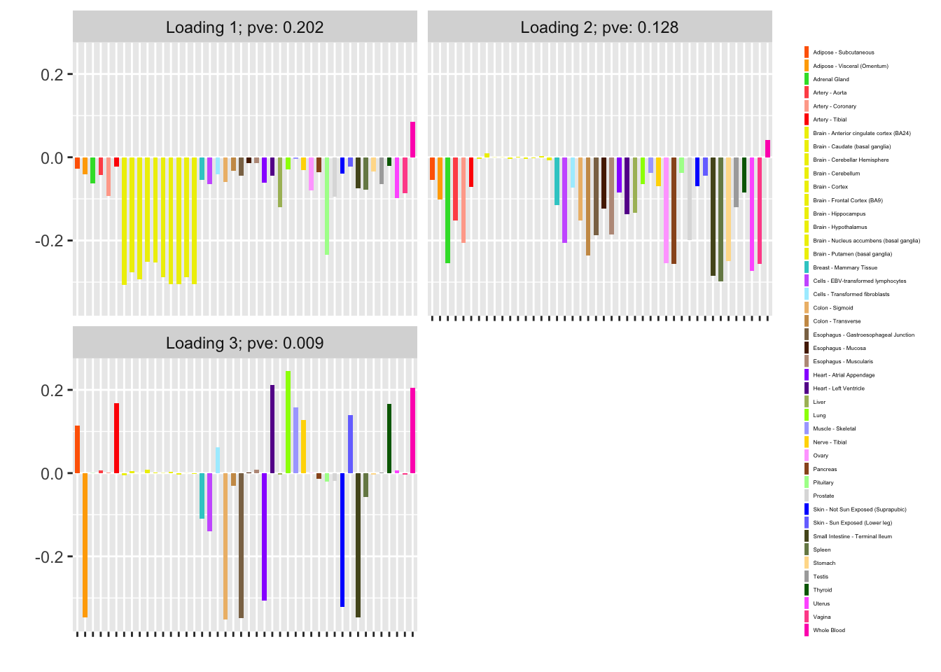
#> Iteration 14: -15486.6758741976I now examine the resulting loadings. One loading primarily represents correlation among brain (and pituitary) tissues; the other represents correlations among the remaining tissues.
plot(fl, plot_loadings = TRUE, loading_colors = gtex.colors,
     loading_legend_size = 3)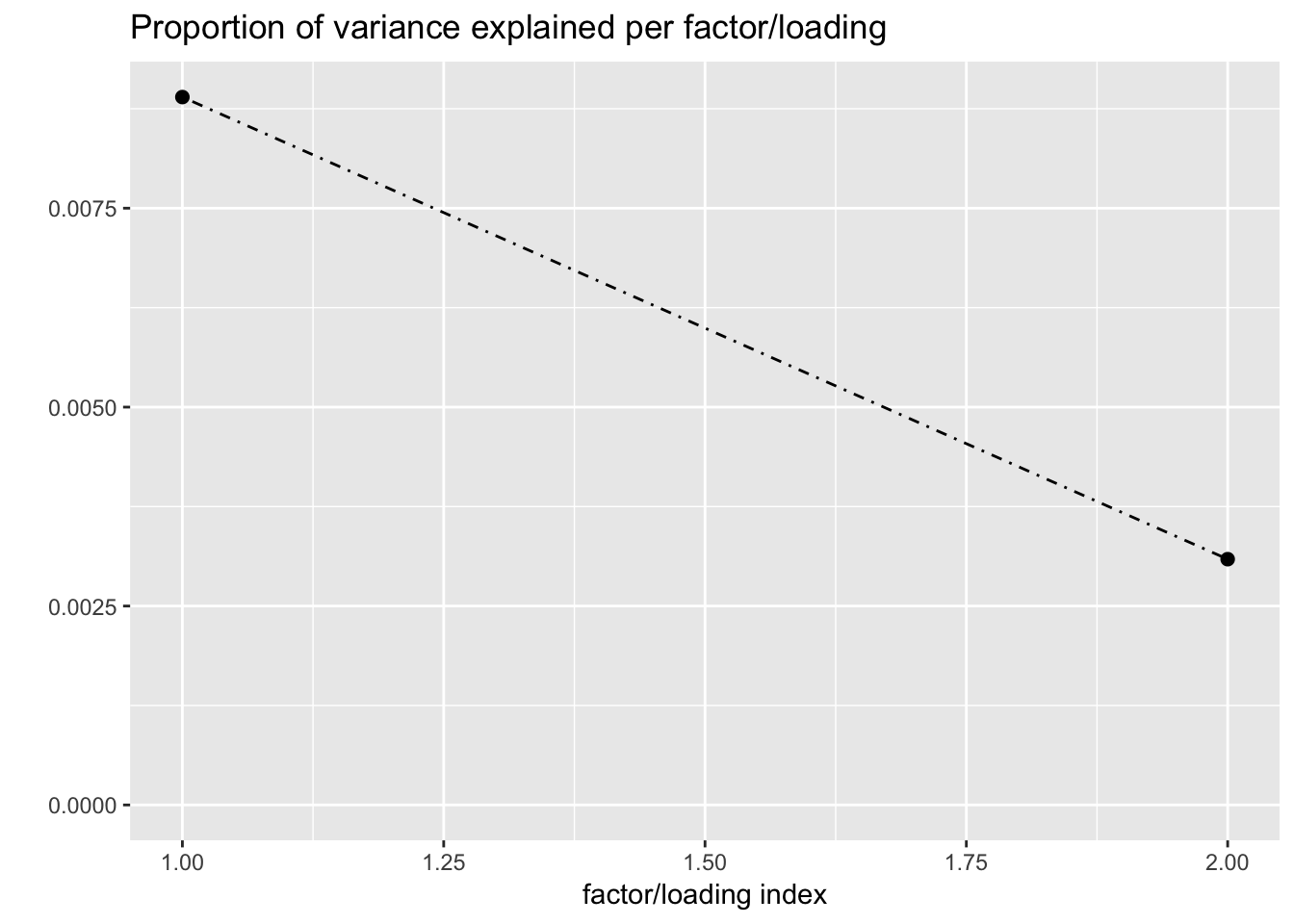
Fitting the model
It is not necessary to run FLASH to convergence before updating \(\mu^\star\). At the extreme, one could do a single FLASH iteration, then update \(\mu^\star\), then run a second FLASH iteration beginning from the updated \(\mu^\star\), and so on.
In the following experiment, I vary the maximum number of iterations between updates of \(\mu^\star\) (n_subiter) from 1 to 100 (which is typically enough to achieve convergence). In each case, I greedily add as many factors as possible and then backfit (as in the above example). I track the final objective attained and the time required to fit (in seconds).
flash_fit <- function(the_data, n_subiter, nonnegative = FALSE,
                      maxiter = 100, tol = .01) {
  fl <- run_one_fit(the_data, f_init = NULL, greedy = TRUE,
                    maxiter = maxiter, n_subiter = n_subiter,
                    nonnegative = nonnegative, verbose = FALSE)
  old_obj <- pois_obj(the_data, fl)

  # Keep greedily adding factors until the objective no longer improves:
  diff <- Inf
  while (diff > tol) {
    fl <- run_one_fit(the_data, fl, greedy = TRUE,
                      maxiter = maxiter, n_subiter = n_subiter,
                      nonnegative = nonnegative, verbose = FALSE)
    new_obj <- pois_obj(the_data, fl)
    diff <- new_obj - old_obj
    old_obj <- new_obj
  }

  # Now backfit the whole thing:
  fl <- run_one_fit(the_data, fl, greedy = FALSE,
                    maxiter = maxiter, n_subiter = n_subiter,
                    nonnegative = nonnegative, verbose = FALSE)

  return(fl)
}

n_subiters <- c(1, 2, 5, 10, 25, 50, 100)
all_t <- rep(0, length(n_subiters))
all_obj <- rep(0, length(n_subiters))
for (i in 1:length(n_subiters)) {
  t <- system.time(fl <- flash_fit(data, n_subiters[i]))
  all_t[i] <- t[3]
  all_obj[i] <- pois_obj(data, fl)
}

df <- data.frame(n_subiter = n_subiters,
                 "time to fit" = all_t,
                 "final objective" = all_obj)
knitr::kable(df)| n_subiter | time.to.fit | final.objective |
|---|---|---|
| 1 | 6.776 | -15536.72 |
| 2 | 7.296 | -15486.69 |
| 5 | 8.562 | -15486.61 |
| 10 | 12.067 | -15486.67 |
| 25 | 12.285 | -15486.67 |
| 50 | 12.500 | -15486.68 |
| 100 | 12.006 | -15486.68 |
Clearly, capping the number of iterations per FLASH fit reduces overall fitting time. It is possible that too few iterations produces a suboptimal fit (the objective for n_subiter = 1 is about 50 less than the other objectives), but this could be an isolated event.
Nonnegative loadings
Since, as I’ve argued in other analyses, putting nonnegative constraints on the loadings helps produce more interpretable factors, I repeat the above experiment with nonnegative “+uniform” priors on the loadings.
for (i in 1:length(n_subiters)) {
  t <- system.time(fl <- flash_fit(data, n_subiters[i],
                                   nonnegative = TRUE))
  all_t[i] <- t[3]
  all_obj[i] <- pois_obj(data, fl)
}

nonneg_df <- data.frame(n_subiter = n_subiters,
                 "time to fit (seconds)" = all_t,
                 "final objective" = all_obj)
knitr::kable(nonneg_df)| n_subiter | time.to.fit..seconds. | final.objective |
|---|---|---|
| 1 | 5.489 | -15344.47 |
| 2 | 7.974 | -15372.43 |
| 5 | 9.064 | -15372.43 |
| 10 | 10.744 | -15372.43 |
| 25 | 10.687 | -15372.43 |
| 50 | 11.182 | -15372.43 |
| 100 | 14.260 | -15372.43 |
Again, the objective for n_subiter = 1 is much different from other settings of n_subiter, but here it is almost 30 higher!
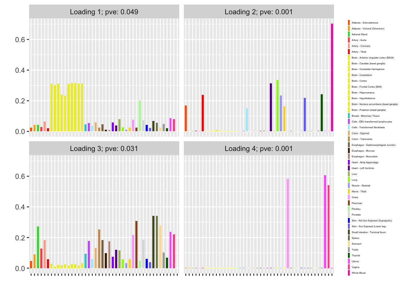
Finally, I refit with n_subiter = 1 and then do a second round of greedily adding factors and backfitting. Doing so yields a fourth factor, which is almost exclusively loaded on female reproductive tissues. (Further rounds of greedy addition and backfitting do not yield any additional factors.)
fl <- flash_fit(data, 1, TRUE)
# The last factor is essentially estimated at zero and can be
#   removed:
fl <- flash_zero_out_factor(data, fl, fl$nfactors)

fl <- run_one_fit(data, fl, greedy = TRUE, n_subiter = 1,
                  nonnegative = TRUE)
#> Iteration 1: -15311.1586217644
#> Iteration 2: -15310.5323444785
#> Iteration 3: -15310.4589463848
#> Iteration 4: -15310.4512300467
fl <- run_one_fit(data, fl, greedy = TRUE, n_subiter = 1,
                  nonnegative = TRUE)
#> Iteration 1: -15310.4503445395
#> Iteration 2: -15310.4502385985
fl <- run_one_fit(data, fl, greedy = FALSE, n_subiter = 1,
                  nonnegative = TRUE)
#> Iteration 1: -15380.2304424497
#> Iteration 2: -15295.7655804381
#> Iteration 3: -15375.9859590359
#> Iteration 4: -15296.9073559686
#> Iteration 5: -15377.713963442
#> Iteration 6: -15298.5612779106
#> Iteration 7: -15378.9404559287
#> Iteration 8: -15299.3185494194
#> Iteration 9: -15379.2021010649
#> Iteration 10: -15299.4879464561
#> Iteration 11: -15379.2647876735
#> Iteration 12: -15299.5443290732
#> Iteration 13: -15379.2881118523
#> Iteration 14: -15299.5821654482
#> Iteration 15: -15379.3057886143
#> Iteration 16: -15299.6097381597
#> Iteration 17: -15379.3185673261
#> Iteration 18: -15299.6279756113
#> Iteration 19: -15379.3266285125

plot(fl, plot_loadings = TRUE, loading_colors = gtex.colors,
     loading_legend_size = 3)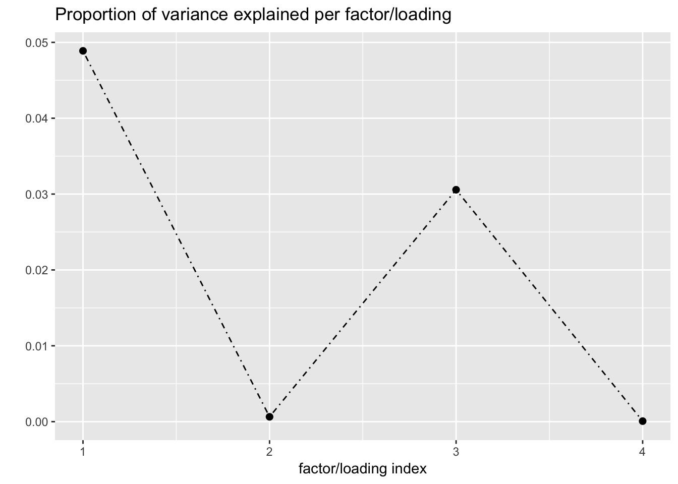
A streamlined approach
It might be worth it to try to streamline the approach by getting a good initialization point, running FLASH a single time to update \(\mu^\star\), and then forgetting about the original data entirely.
I obtain an initialization point by running nonnegative FLASH on the data (recall that \(\mu^\star\) must be strictly positive).
t_init <- system.time(
  fl <- suppressWarnings(
    flash(data, var_type = "by_row", ebnm_fn = "ebnm_ash",
          ebnm_param = list(mixcompdist = "+uniform"),
          verbose = FALSE)
  )
)
mu <- fl$fitted_values
Note that this takes about as long as the entire fitting process with n_subiter = 1 above!
round(t_init[3], digits = 2)
#> elapsed
#>    7.88
Now I run FLASH on the pseudo-data and update \(\mu^\star\):
pseudodata <- set_pseudodata(data, mu)
t_update <- system.time(
  fl <- suppressWarnings(
    flash(pseudodata, var_type = "zero", backfit = TRUE,
          verbose = FALSE)
  )
)
mu <- exp(fl$fitted_values)
round(t_update[3], digits = 2)
#> elapsed
#>    5.03
pseudodata <- set_pseudodata(data, mu)
t_final <- system.time(
fl <- suppressWarnings(
flash(pseudodata, var_type = "zero", backfit = TRUE,
verbose = FALSE)
)
)
round(t_final[3], digits = 2)
#> elapsed
#> 4.96The objective is not much worse than the the objective attained using the more involved approach above (it is about 70 lower):
pois_obj(data, fl)
#> [1] -15588
However, the loadings tell a somewhat different story:
plot(fl, plot_loadings = TRUE, loading_colors = gtex.colors,
     loading_legend_size = 3)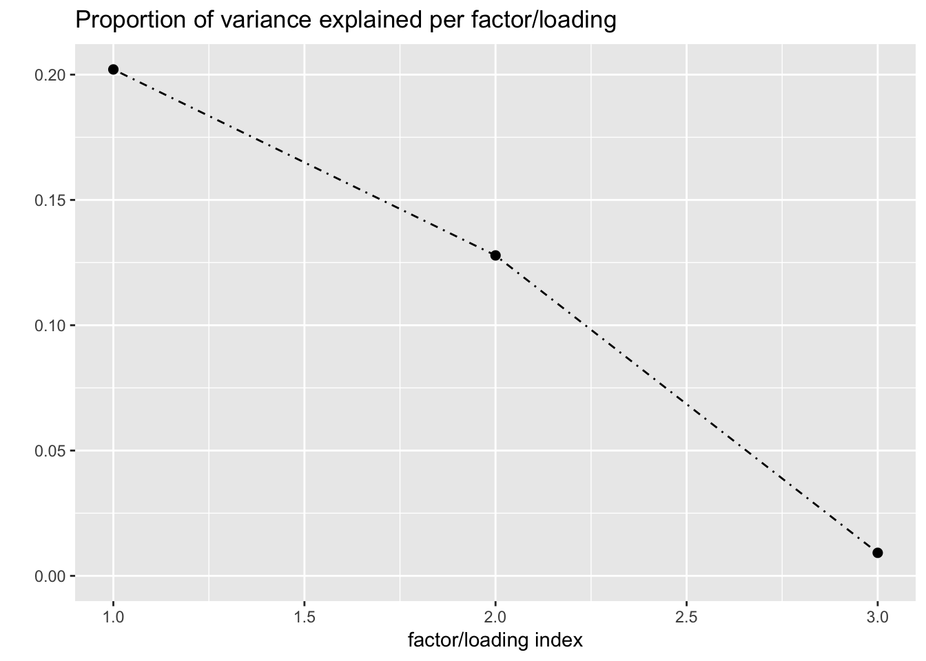
Further, this simpler approach is slower than the above approach for all values of n_subiter:
round(t_init[3] + t_update[3] + t_final[3], digits = 2)
#> elapsed
#>   17.87
Session information
sessionInfo()
#> R version 3.4.3 (2017-11-30)
#> Platform: x86_64-apple-darwin15.6.0 (64-bit)
#> Running under: macOS High Sierra 10.13.6
#>
#> Matrix products: default
#> BLAS: /Library/Frameworks/R.framework/Versions/3.4/Resources/lib/libRblas.0.dylib
#> LAPACK: /Library/Frameworks/R.framework/Versions/3.4/Resources/lib/libRlapack.dylib
#>
#> locale:
#> [1] en_US.UTF-8/en_US.UTF-8/en_US.UTF-8/C/en_US.UTF-8/en_US.UTF-8
#>
#> attached base packages:
#> [1] stats     graphics  grDevices utils     datasets  methods   base
#>
#> other attached packages:
#> [1] ebnm_0.1-14  flashr_0.6-1
#>
#> loaded via a namespace (and not attached):
#>  [1] Rcpp_0.12.18        highr_0.6           pillar_1.2.1
#>  [4] plyr_1.8.4          compiler_3.4.3      git2r_0.21.0
#>  [7] workflowr_1.0.1     R.methodsS3_1.7.1   R.utils_2.6.0
#> [10] iterators_1.0.9     tools_3.4.3         testthat_2.0.0
#> [13] digest_0.6.15       tibble_1.4.2        evaluate_0.10.1
#> [16] memoise_1.1.0       gtable_0.2.0        lattice_0.20-35
#> [19] rlang_0.2.0         Matrix_1.2-12       foreach_1.4.4
#> [22] commonmark_1.4      yaml_2.1.17         parallel_3.4.3
#> [25] withr_2.1.1.9000    stringr_1.3.0       roxygen2_6.0.1.9000
#> [28] xml2_1.2.0          knitr_1.20          REBayes_1.2
#> [31] devtools_1.13.4     rprojroot_1.3-2     grid_3.4.3
#> [34] R6_2.2.2            rmarkdown_1.8       reshape2_1.4.3
#> [37] ggplot2_2.2.1       ashr_2.2-13         magrittr_1.5
#> [40] whisker_0.3-2       backports_1.1.2     scales_0.5.0
#> [43] codetools_0.2-15    htmltools_0.3.6     MASS_7.3-48
#> [46] assertthat_0.2.0    softImpute_1.4      colorspace_1.3-2
#> [49] labeling_0.3        stringi_1.1.6       Rmosek_7.1.3
#> [52] lazyeval_0.2.1      doParallel_1.0.11   pscl_1.5.2
#> [55] munsell_0.4.3       truncnorm_1.0-8     SQUAREM_2017.10-1
#> [58] R.oo_1.21.0
This reproducible R Markdown analysis was created with workflowr 1.0.1