Gaussian mean estimation in simulated data sets

Set up environment

Load the ggplot2 and cowplot packages, and the functions definining the mean and variances used to simulate the data.

library(ggplot2)
# Warning: package 'ggplot2' was built under R version 3.4.4
library(cowplot)
# Warning: package 'cowplot' was built under R version 3.4.4
# 
# Attaching package: 'cowplot'
# The following object is masked from 'package:ggplot2':
# 
#     ggsave
source("../code/signals.R")

Load results

Load the results of the simulation experiments.

load("../output/gaus-dscr.RData")

Summarize results on data sets with constant variances

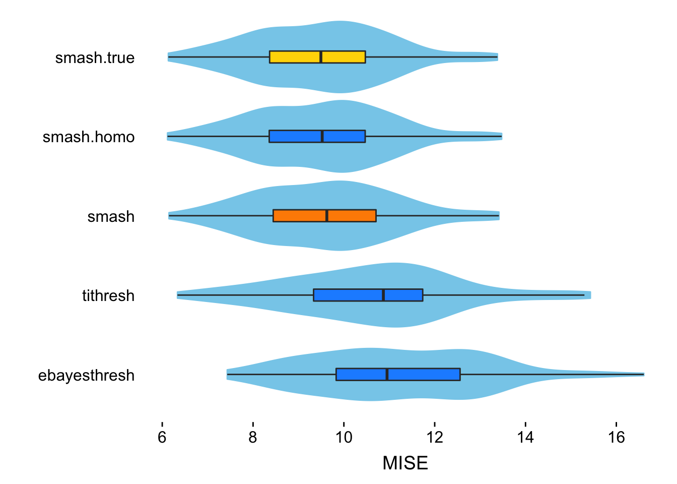
This plot reproduces Fig. 2 of the manuscript comparing the accuracy of estimated mean curves in the data sets simulated from the “Spikes” mean function with constant variance.

First extract the data used to generate this plot.

homo.data.smash <-
  res[res$.id    == "sp.3.v1" &
      res$method == "smash.s8",]
homo.data.smash.homo <-
  res[res$.id    == "sp.3.v1" &
      res$method == "smash.homo.s8",]
homo.data.tithresh <-
  res[res$.id == "sp.3.v1" &
      res$method == "tithresh.homo.s8",]
homo.data.ebayes <-
  res[res$.id    == "sp.3.v1" &
      res$method == "ebayesthresh",]
homo.data.smash.true <-
  res[res$.id == "sp.3.v1" &
  res$method  == "smash.true.s8",]
homo.data <-
  res[res$.id == "sp.3.v1" &
  (res$method == "smash.s8" |
   res$method == "ebayesthresh" |
   res$method == "tithresh.homo.s8"),]

Transform these data into a data frame suitable for ggplot2.

pdat <-
  rbind(data.frame(method      = "smash",
                   method.type = "est",
                   mise        = homo.data.smash$mise),
        data.frame(method      = "smash.homo",
                   method.type = "homo",
                   mise        = homo.data.smash.homo$mise),
        data.frame(method      = "tithresh",
                   method.type = "homo",
                   mise        = homo.data.tithresh$mise),
        data.frame(method      = "ebayesthresh",
                   method.type = "homo",
                   mise        = homo.data.ebayes$mise),
        data.frame(method      = "smash.true",
                   method.type = "true",
                   mise        = homo.data.smash.true$mise))
pdat <-
  transform(pdat,
            method = factor(method,
                            names(sort(tapply(pdat$mise,pdat$method,mean),
                                       decreasing = TRUE))))

Create the combined boxplot and violin plot using ggplot2.

p <- ggplot(pdat,aes(x = method,y = mise,fill = method.type)) +
     geom_violin(fill = "skyblue",color = "skyblue") +
     geom_boxplot(width = 0.15,outlier.shape = NA) +
     scale_y_continuous(breaks = seq(6,16,2)) +
     scale_fill_manual(values = c("darkorange","dodgerblue","gold"),
                       guide = FALSE) +
     coord_flip() +
     labs(x = "",y = "MISE") +
     theme(axis.line = element_blank(),
           axis.ticks.y = element_blank())
print(p)

Session information

sessionInfo()
# R version 3.4.3 (2017-11-30)
# Platform: x86_64-apple-darwin15.6.0 (64-bit)
# Running under: macOS High Sierra 10.13.6
# 
# Matrix products: default
# BLAS: /Library/Frameworks/R.framework/Versions/3.4/Resources/lib/libRblas.0.dylib
# LAPACK: /Library/Frameworks/R.framework/Versions/3.4/Resources/lib/libRlapack.dylib
# 
# locale:
# [1] en_US.UTF-8/en_US.UTF-8/en_US.UTF-8/C/en_US.UTF-8/en_US.UTF-8
# 
# attached base packages:
# [1] stats     graphics  grDevices utils     datasets  methods   base     
# 
# other attached packages:
# [1] cowplot_0.9.3 ggplot2_3.0.0
# 
# loaded via a namespace (and not attached):
#  [1] Rcpp_0.12.18      later_0.7.2       dscr_0.1-7       
#  [4] compiler_3.4.3    pillar_1.2.1      git2r_0.21.0     
#  [7] plyr_1.8.4        workflowr_1.1.1   bindr_0.1.1      
# [10] R.methodsS3_1.7.1 R.utils_2.6.0     tools_3.4.3      
# [13] digest_0.6.16     evaluate_0.10.1   tibble_1.4.2     
# [16] gtable_0.2.0      pkgconfig_2.0.1   rlang_0.2.1      
# [19] shiny_1.1.0       yaml_2.2.0        bindrcpp_0.2.2   
# [22] withr_2.1.2       stringr_1.3.0     dplyr_0.7.5      
# [25] knitr_1.20        rprojroot_1.3-2   grid_3.4.3       
# [28] tidyselect_0.2.4  glue_1.2.0        R6_2.2.2         
# [31] rmarkdown_1.9     purrr_0.2.5       magrittr_1.5     
# [34] whisker_0.3-2     promises_1.0.1    backports_1.1.2  
# [37] scales_0.5.0      htmltools_0.3.6   assertthat_0.2.0 
# [40] xtable_1.8-2      mime_0.5          colorspace_1.4-0 
# [43] httpuv_1.4.3      stringi_1.1.7     lazyeval_0.2.1   
# [46] munsell_0.4.3     R.oo_1.21.0