Spikes demo

Set up environment

We begin by loading the ashr, smashr, scales, ggplot2 and cowplot packages, as well as some additional functions used in the code below.

library(ashr)
library(smashr)
library(scales)
library(ggplot2)

Warning: package 'ggplot2' was built under R version 3.4.4

suppressMessages(library(cowplot))

Warning: package 'cowplot' was built under R version 3.4.4

source("../code/misc.R")

Define the “spikes” mean function

Function spike.f defines the mean signal.

n <- 1024
t <- 1:n/n
spike.f <-
  function (x) (0.75 * exp(-500   * (x - 0.23)^2) +
                1.5  * exp(-2000  * (x - 0.33)^2) +
                3    * exp(-8000  * (x - 0.47)^2) +
                2.25 * exp(-16000 * (x - 0.69)^2) +
                0.5  * exp(-32000 * (x - 0.83)^2))
mu.sp <- spike.f(t)
mu.sp <- (1 + mu.sp)/5

Simulate data

Add text here.

pos <- c(0.1,0.13,0.15,0.23,0.25,0.4,0.44,0.65,0.76,0.78,0.81)
hgt <- 2.88/5 * c(4,-5,3,-4,5,-4.2,2.1,4.3,-3.1,2.1,-4.2)
sig.cb <- rep(0,length(t))
for (j in 1:length(pos)) 
  sig.cb <- sig.cb + (1 + sign(t - pos[j])) * (hgt[j]/2)
sig.cb[sig.cb < 0] <- 0
sig.cb <- 0.1 + (sig.cb - min(sig.cb))/max(sig.cb)
rsnr   <- sqrt(3)
sig.cb <- sig.cb/mean(sig.cb) * sd(mu.sp)/rsnr^2
x.sim  <- rnorm(n,mu.sp,sig.cb)

Plot the simulated data set.

par(cex.axis = 0.8,cex.sub = 1,cex.lab = 1)
plot(mu.sp,type = 'l',ylim = c(-0.05,1),xlab = "position",
     ylab = "",lwd = 1.7,xaxp = c(0,1024,4),yaxp = c(0,1,4))
lines(mu.sp + 2*sig.cb,col = "darkorange",lty = 5,lwd = 1.8)
lines(mu.sp - 2*sig.cb,col = "darkorange",lty = 5,lwd = 1.8)
points(x.sim,cex = 0.7,pch = 16,col = "darkblue")

Run SMASH and TI thresholding

Apply smash and translation invariant (TI) thresholding to the “spikes” data. Here, we run the TI thresholding twice—once when the standard deviation (s.d.) function is provided, and once when it is estimated using the MAD algorithm.

sig.est  <- sqrt(2/(3 * (n - 2)) *
                 sum((1/2 * x.sim[1:(n-2)] - x.sim[2:(n-1)] + x.sim[3:n])^2/2))
mu.smash <- smash(x.sim,family = "DaubLeAsymm",filter.number = 8)
mu.ti    <- ti.thresh(x.sim,method = "rmad",family = "DaubLeAsymm",
                      filter.number = 8)
mu.ti.homo <- ti.thresh(x.sim,sigma = sig.est,family = "DaubLeAsymm",
                        filter.number = 8)

Get the wavelet coefficients and their variances.

wc.sim     <- titable(x.sim)$difftable
wc.var.sim <- titable(sig.cb^2)$sumtable
wc.true    <- titable(mu.sp)$difftable

Get shrunken estimates of the wavelet coefficients.

wc.sim.shrunk <- vector("list",10)
wc.pres       <- vector("list",10)
for(j in 0:(log2(n) - 1)){
  wc.sim.shrunk[[j+1]] <-
    ash(wc.sim[j+2,],sqrt(wc.var.sim[j+2,]),prior = "nullbiased",
        pointmass = TRUE,mixsd = NULL,mixcompdist = "normal",
        gridmult = 2,df = NULL)$result
  wc.pres[[j+1]] <- 1/sqrt(wc.var.sim[j+2,])
}

Summarize results

Plot the distribution of observed wavelet coefficients.

par(cex.axis = 0.8,cex.lab = 0.8)
hist(wc.sim[4,],breaks = 2,xlab = "observed wavelet coefficients",
     xlim = c(-25,25),ylim = c(0,600),col = "darkblue",xaxp = c(-25,25,10),
     yaxp = c(0,600,6),main = "")
hist(wc.sim[10,],breaks = 40,add = TRUE,col = "darkorange")

Plot the observed wavelet coefficients (at scales 1 and 7 only) vs. the “shrunken” wavelet coefficients estimated by adaptive shrinkage.

par(cex.axis = 0.8,cex.lab = 0.8)
plot(c(),c(),xlab = "observed wavelet coefficients",
     ylab = "shrunken wavelet coefficients",
     xlim = c(-2.5,2.5),ylim = c(-2.5,2.5))
abline(0,1,lty = 1,col = "gray",lwd = 1)
points(wc.sim[10,],wc.sim.shrunk[[9]]$PosteriorMean,pch = 20,cex = 0.6,
       col = "darkorange")
points(wc.sim[4,],wc.sim.shrunk[[3]]$PosteriorMean,pch = 20,cex = 0.6,
       col = "darkblue")

Plot the observed wavelet coefficients (at scale 7 only) vs. the “shrunken” wavelet coefficients estimated by adaptive shrinkage, and how how the amount of shrinkage depends on the standard error (s.e.) in the observations.

wc.sig.3 <- 1/wc.pres[[3]]
p <- ggplot(data.frame(observed = wc.sim[4,],
                       shrunken = wc.sim.shrunk[[3]]$PosteriorMean,
                       se       = wc.sig.3),
            aes(x = observed,y = shrunken,col = se)) +
  geom_point() +
  xlim(c(-1,1)) +
  ylim(c(-1,1)) +
  scale_color_gradientn(colors = c("deepskyblue","darkblue")) +
  theme_cowplot()
print(p)

Warning: Removed 3 rows containing missing values (geom_point).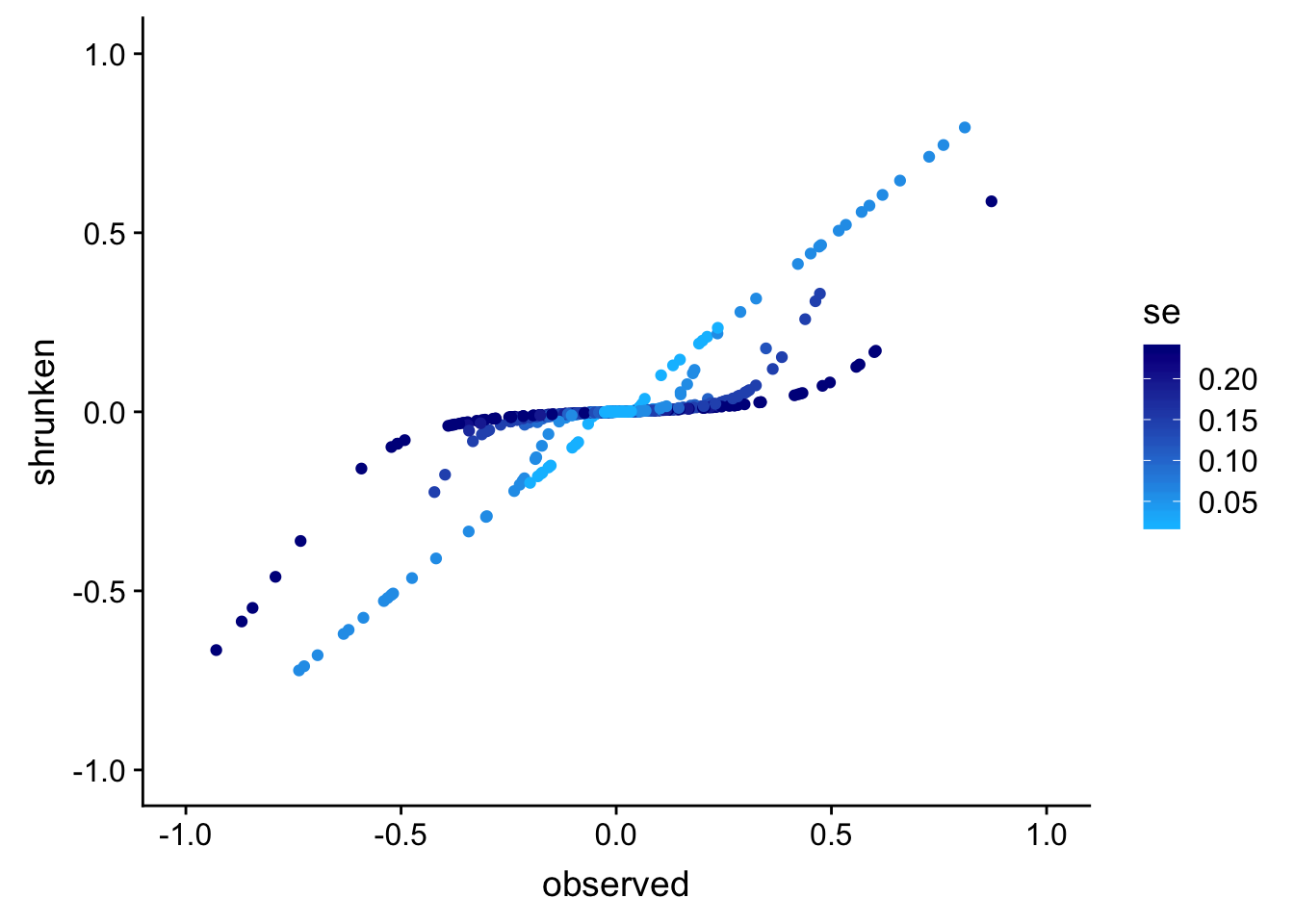

Plot the ground-truth signal (mean function) and the signals recovered by the TI thresholding and smash methods.

par(cex.axis = 0.8)
plot(mu.sp,type = "l",col = "black",lwd = 2,xlab = "position",ylab = "",
     ylim = c(-0.05,1),xaxp = c(0,1024,4),yaxp = c(0,1,4))
lines(mu.ti,col = "dodgerblue",lwd = 1.5)
lines(mu.smash,col = "orangered",lwd = 1.5)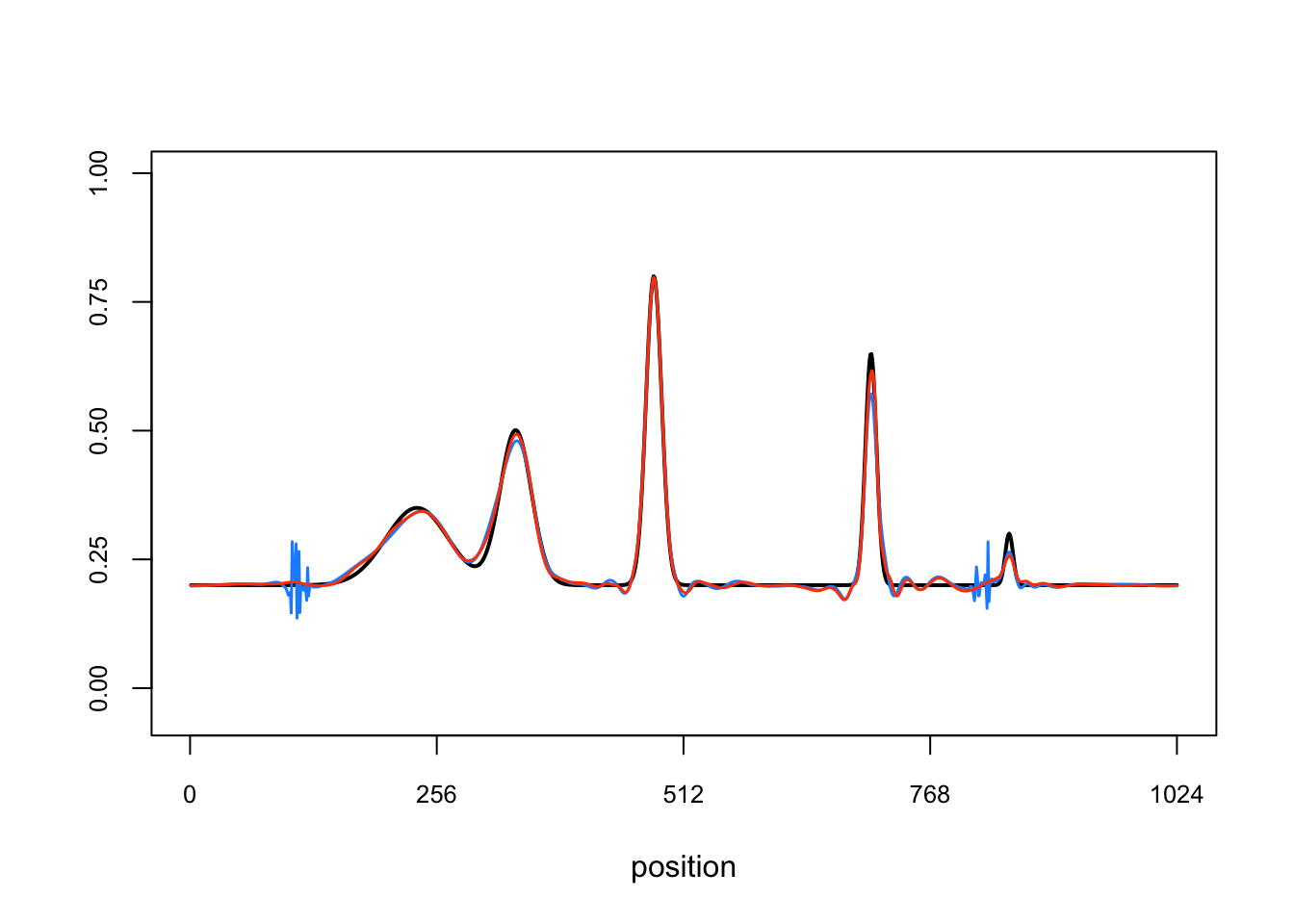

cat("Demo is over.\n")

Demo is over.

Session information

sessionInfo()

R version 3.4.3 (2017-11-30)
Platform: x86_64-apple-darwin15.6.0 (64-bit)
Running under: macOS High Sierra 10.13.6

Matrix products: default
BLAS: /Library/Frameworks/R.framework/Versions/3.4/Resources/lib/libRblas.0.dylib
LAPACK: /Library/Frameworks/R.framework/Versions/3.4/Resources/lib/libRlapack.dylib

locale:
[1] en_US.UTF-8/en_US.UTF-8/en_US.UTF-8/C/en_US.UTF-8/en_US.UTF-8

attached base packages:
[1] stats     graphics  grDevices utils     datasets  methods   base     

other attached packages:
[1] cowplot_0.9.3 ggplot2_3.0.0 scales_0.5.0  smashr_1.2-0  ashr_2.2-9   

loaded via a namespace (and not attached):
 [1] wavethresh_4.6.8  tidyselect_0.2.4  purrr_0.2.5      
 [4] lattice_0.20-35   Rmosek_8.0.69     colorspace_1.4-0 
 [7] htmltools_0.3.6   yaml_2.1.19       rlang_0.2.1      
[10] R.oo_1.21.0       pillar_1.2.1      glue_1.2.0       
[13] withr_2.1.2       R.utils_2.6.0     REBayes_1.3      
[16] bindrcpp_0.2.2    foreach_1.4.4     plyr_1.8.4       
[19] bindr_0.1.1       stringr_1.3.0     munsell_0.4.3    
[22] gtable_0.2.0      workflowr_1.1.1   R.methodsS3_1.7.1
[25] caTools_1.17.1    codetools_0.2-15  evaluate_0.10.1  
[28] labeling_0.3      knitr_1.20        pscl_1.5.2       
[31] doParallel_1.0.11 parallel_3.4.3    Rcpp_0.12.17     
[34] backports_1.1.2   truncnorm_1.0-8   digest_0.6.15    
[37] stringi_1.1.7     dplyr_0.7.5       grid_3.4.3       
[40] rprojroot_1.3-2   tools_3.4.3       bitops_1.0-6     
[43] magrittr_1.5      lazyeval_0.2.1    tibble_1.4.2     
[46] whisker_0.3-2     pkgconfig_2.0.1   MASS_7.3-48      
[49] Matrix_1.2-12     SQUAREM_2017.10-1 data.table_1.11.4
[52] mixSQP_0.1-6      assertthat_0.2.0  rmarkdown_1.9    
[55] iterators_1.0.9   R6_2.2.2          git2r_0.21.0     
[58] compiler_3.4.3