Examples illustrating how mash uses patterns of sharing to inform effect estimates
Sarah Urbut, Gao Wang, Peter Carbonetto and Matthew Stephens
Last updated: 2018-06-05
workflowr checks: (Click a bullet for more information)-
✔ R Markdown file: up-to-date
Great! Since the R Markdown file has been committed to the Git repository, you know the exact version of the code that produced these results.
-
✔ Environment: empty
Great job! The global environment was empty. Objects defined in the global environment can affect the analysis in your R Markdown file in unknown ways. For reproduciblity it’s best to always run the code in an empty environment.
-
✔ Seed:
set.seed(1)The command
set.seed(1)was run prior to running the code in the R Markdown file. Setting a seed ensures that any results that rely on randomness, e.g. subsampling or permutations, are reproducible. -
✔ Session information: recorded
Great job! Recording the operating system, R version, and package versions is critical for reproducibility.
-
Great! You are using Git for version control. Tracking code development and connecting the code version to the results is critical for reproducibility. The version displayed above was the version of the Git repository at the time these results were generated.✔ Repository version: 87df348
Note that you need to be careful to ensure that all relevant files for the analysis have been committed to Git prior to generating the results (you can usewflow_publishorwflow_git_commit). workflowr only checks the R Markdown file, but you know if there are other scripts or data files that it depends on. Below is the status of the Git repository when the results were generated:
Note that any generated files, e.g. HTML, png, CSS, etc., are not included in this status report because it is ok for generated content to have uncommitted changes.Ignored files: Ignored: .sos/ Ignored: data/.sos/ Ignored: output/MatrixEQTLSumStats.Portable.Z.coved.K3.P3.lite.single.expanded.V1.loglik.rds Ignored: workflows/.ipynb_checkpoints/ Ignored: workflows/.sos/ Untracked files: Untracked: TODO.txt Untracked: analysis/files.txt Untracked: fastqtl_to_mash_output/ Untracked: gtex6_workflow_output/ Unstaged changes: Modified: analysis/gtex.Rmd
Expand here to see past versions:
Having estimated patterns of sharing from the data, mash exploits these patterns to improve effect estimates at each putative eQTL. Here we give three examples can provide intuition into the way that mash achieves improved accuracy of effect estimation.
Compare the plots against Figure 4 of the paper.
Set up environment
First, we load the rmeta package, as well as some functions defined for mash analyses.
source("../code/normfuncs.R")
library(rmeta)
Load data and mash results
In the next code chunk, we load some GTEx summary statistics, as well as some of the results generated from the mash analysis of the GTEx data.
out    <- readRDS("../data/MatrixEQTLSumStats.Portable.Z.rds")
b.stat <- out$test.b
z.stat <- out$test.z
out    <- readRDS(paste("../output/MatrixEQTLSumStats.Portable.Z.coved.K3.P3",
                        "lite.single.expanded.V1.posterior.rds",sep = "."))
posterior.means <- out$posterior.means
lfsr            <- out$lfsr
mar.var         <- out$marginal.var
rm(out)
colnames(lfsr)  <-
  colnames(mar.var) <-
  colnames(posterior.means) <-
  colnames(z.stat)
standard.error  <- b.stat/z.stat
posterior.betas <- standard.error * posterior.means
pm.beta.norm    <- het.norm(posterior.betas)
Load the tissue indices:
missing.tissues <- c(7,8,19,20,24,25,31,34,37)
uk3labels       <- read.table("../data/uk3rowindices.txt")[,1]
For the plots of the eigenvectors, we load the colours that are conventionally used to represent the tissues in plots.
gtex.colors <- read.table('../data/GTExColors.txt', sep = '\t',
                          comment.char = '')[-missing.tissues,2]
gtex.colors <- gtex.colors[uk3labels]
MCPH1 gene
In the first example, the vast majority of effect estimates are positive in each tissue, with the strongest signals in a subset of brain tissues. Based on the patterns of sharing learned in the first step, mash estimates the effects in all tissues to be positive—even those with negative observed effects. This is because the few modest negative effects at this eQTL are outweighed by the strong background information that effects are highly correlated among tissues.
To create the metaplot, we first define a function which we will use in this example, and reuse in subsequent examples.
create.metaplot <- function (j) {

  pm.beta.norm  <- pm.beta.norm[,uk3labels] # Shuffle columns.
  z.shuffle     <- z.stat[,uk3labels]
  b.shuffle     <- b.stat[,uk3labels]
  post.var      <- mar.var[,uk3labels]
  post.bshuffle <- posterior.betas[,uk3labels]
  sem.shuffle   <- standard.error[,uk3labels]
  lfsr          <- lfsr[,uk3labels]
  plot.title    <- strsplit(rownames(z.stat)[j], "[.]")[[1]][1]

  x <- as.numeric(post.bshuffle[j,])

  layout(t(1:2))

  metaplot(as.numeric(b.shuffle[j,]),as.numeric(sem.shuffle[j,]),xlab = "",
           ylab = "",colors = meta.colors(box = as.character(gtex.colors)),
           xlim = c(-1,1))
  title(plot.title)

  # Transform to posterior sd of beta.
  sd <- as.numeric(sem.shuffle[j,]) * sqrt(as.numeric(post.var[j,]))
  metaplot(x,sd,xlab = "",ylab = "",
           colors = meta.colors(box = as.character(gtex.colors)),
           xlim = c(-1,1))
  title(plot.title)
}
Now create the MCHP1 metaplot summarizing the eQTL effect estimates. The original effect estimates are shown on the left-hand side, and the shrunken estimates from mash are shown on the right-hand side.
create.metaplot(which(rownames(z.stat) ==
  "ENSG00000249898.3_8_6521432_T_C_b37"))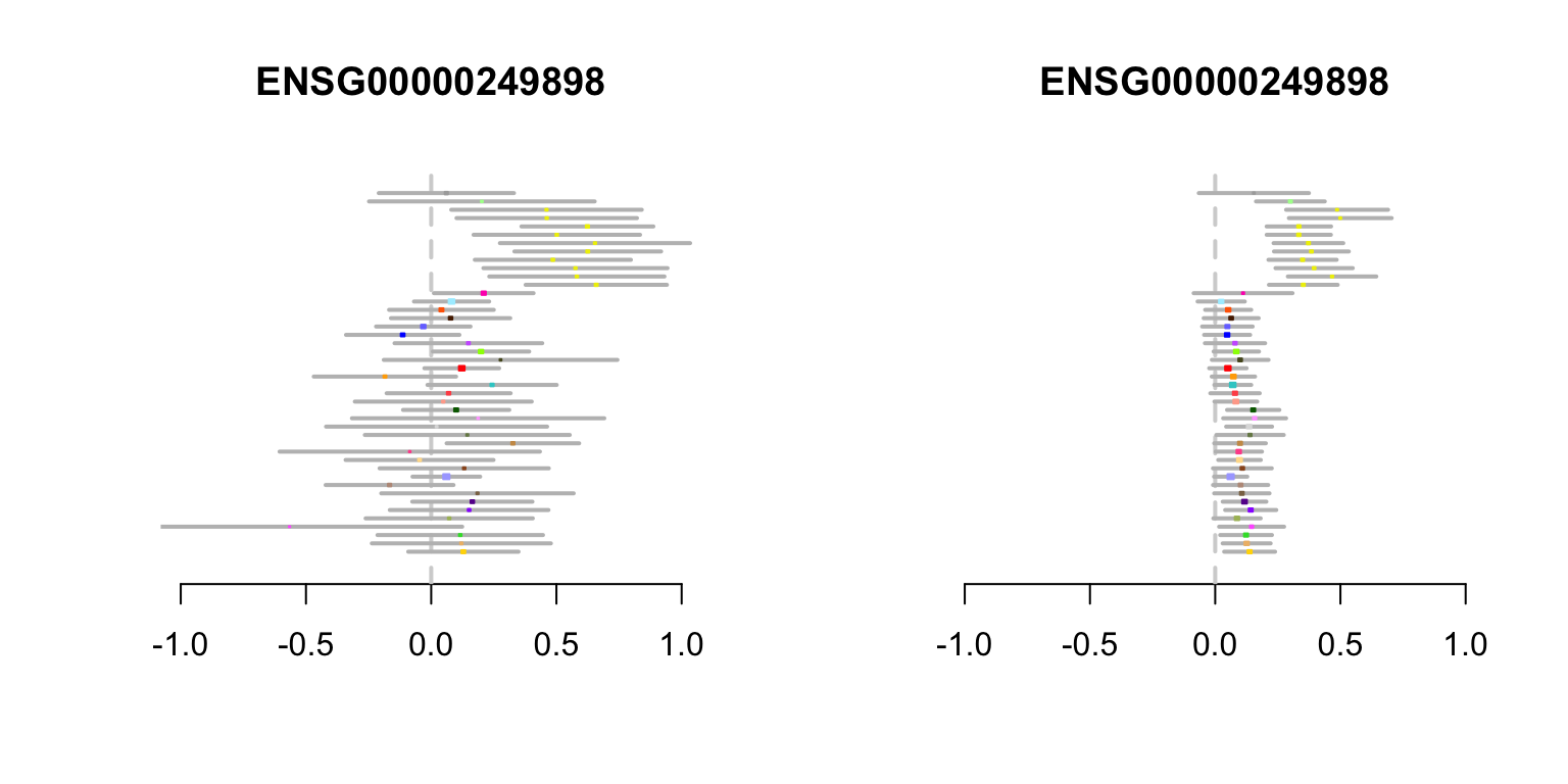
Expand here to see past versions of metaplot-MCPH1-1.png:
| Version | Author | Date |
|---|---|---|
| 12aa3cb | Peter Carbonetto | 2018-06-05 |
FLJ13114 gene
In the second example, the effect estimates in non-brain tissues are mostly positive, but modest in size, and only one effect is, individually, nominally significant. However, combining information among tissues, mash effect estimates in non-brain tissues are all positive, and mostly “significant”.
create.metaplot(which(rownames(z.stat) ==
  "ENSG00000120029.8_10_103924251_G_A_b37"))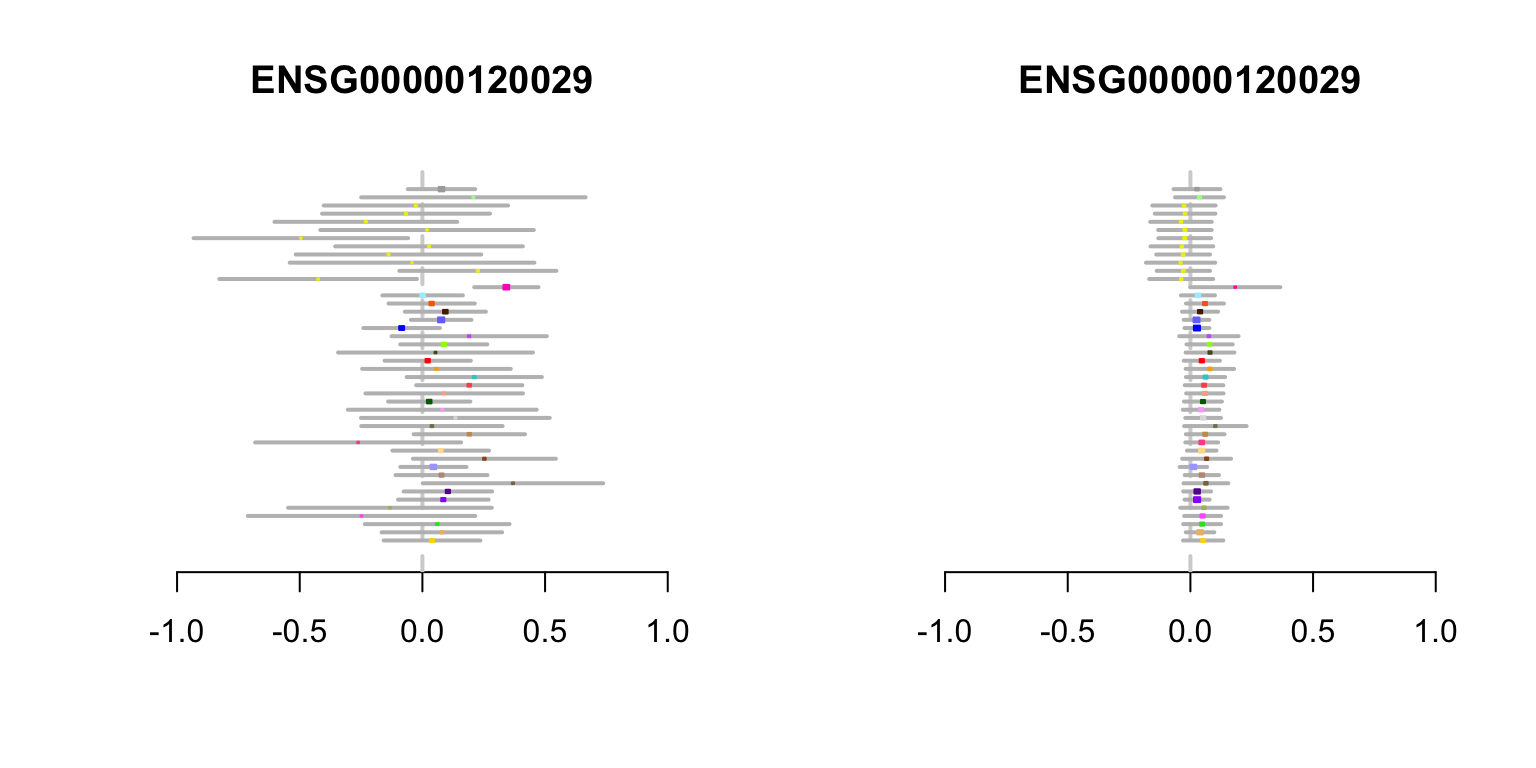
Expand here to see past versions of metaplot-FLJ13114-1.png:
| Version | Author | Date |
|---|---|---|
| 12aa3cb | Peter Carbonetto | 2018-06-05 |
RALBP1 gene
In this example, the effect estimates vary in sign, and are modest except for a very strong signal in whole blood. While whole-blood-specific effects are estimated to be rare, mash recognizes that the strong data at this eQTL outweigh this background information, and estimates a strong effect in blood with insignificant effects in other tissues.
create.metaplot(which(rownames(z.stat) ==
  "ENSG00000017797.7_18_9488704_C_T_b37"))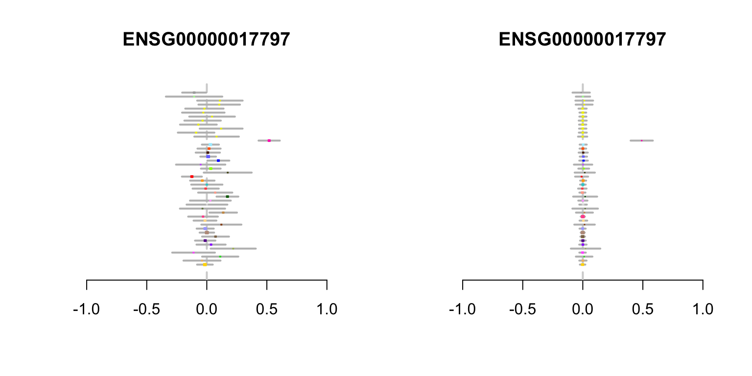
Expand here to see past versions of metaplot-RALBP1-1.png:
| Version | Author | Date |
|---|---|---|
| 12aa3cb | Peter Carbonetto | 2018-06-05 |
Session information
sessionInfo()
# R version 3.4.3 (2017-11-30)
# Platform: x86_64-apple-darwin15.6.0 (64-bit)
# Running under: macOS High Sierra 10.13.4
#
# Matrix products: default
# BLAS: /Library/Frameworks/R.framework/Versions/3.4/Resources/lib/libRblas.0.dylib
# LAPACK: /Library/Frameworks/R.framework/Versions/3.4/Resources/lib/libRlapack.dylib
#
# locale:
# [1] en_US.UTF-8/en_US.UTF-8/en_US.UTF-8/C/en_US.UTF-8/en_US.UTF-8
#
# attached base packages:
# [1] grid      stats     graphics  grDevices utils     datasets  methods
# [8] base
#
# other attached packages:
# [1] rmeta_2.16
#
# loaded via a namespace (and not attached):
#  [1] workflowr_1.0.1.9000 Rcpp_0.12.16         digest_0.6.15
#  [4] rprojroot_1.3-2      R.methodsS3_1.7.1    backports_1.1.2
#  [7] git2r_0.21.0         magrittr_1.5         evaluate_0.10.1
# [10] stringi_1.1.7        whisker_0.3-2        R.oo_1.21.0
# [13] R.utils_2.6.0        rmarkdown_1.9        tools_3.4.3
# [16] stringr_1.3.0        yaml_2.1.18          compiler_3.4.3
# [19] htmltools_0.3.6      knitr_1.20
This reproducible R Markdown analysis was created with workflowr 1.0.1.9000