Number of tissue-specific eQTLs in each tissue
Sarah Urbut, Gao Wang, Peter Carbonetto and Matthew Stephens
Last updated: 2018-06-18
workflowr checks: (Click a bullet for more information)-
✔ R Markdown file: up-to-date
Great! Since the R Markdown file has been committed to the Git repository, you know the exact version of the code that produced these results.
-
✔ Environment: empty
Great job! The global environment was empty. Objects defined in the global environment can affect the analysis in your R Markdown file in unknown ways. For reproduciblity it’s best to always run the code in an empty environment.
-
✔ Seed:
set.seed(1)The command
set.seed(1)was run prior to running the code in the R Markdown file. Setting a seed ensures that any results that rely on randomness, e.g. subsampling or permutations, are reproducible. -
✔ Session information: recorded
Great job! Recording the operating system, R version, and package versions is critical for reproducibility.
-
Great! You are using Git for version control. Tracking code development and connecting the code version to the results is critical for reproducibility. The version displayed above was the version of the Git repository at the time these results were generated.✔ Repository version: 14f28d4
Note that you need to be careful to ensure that all relevant files for the analysis have been committed to Git prior to generating the results (you can usewflow_publishorwflow_git_commit). workflowr only checks the R Markdown file, but you know if there are other scripts or data files that it depends on. Below is the status of the Git repository when the results were generated:
Note that any generated files, e.g. HTML, png, CSS, etc., are not included in this status report because it is ok for generated content to have uncommitted changes.Unstaged changes: Modified: analysis/hettablesim
Expand here to see past versions:
| File | Version | Author | Date | Message |
|---|---|---|---|---|
| Rmd | 6314ce0 | Gao Wang | 2018-06-16 | Relabel ‘test’ to ‘strong’ in data and code |
| html | 6eee6a9 | Peter Carbonetto | 2018-06-06 | Updated the webpages for a bunch of R Markdown files after minor revisions. |
| Rmd | 3dc0ba5 | Peter Carbonetto | 2018-06-06 | wflow_publish(c(“ExpressionAnalysis.Rmd”, “fastqtl2mash.Rmd”, |
| Rmd | 2b0db9b | Peter Carbonetto | 2018-06-06 | Misc. revisions to Rmd files. |
| html | 678f73e | Peter Carbonetto | 2018-06-06 | Added text to Tspecific analysis file. |
| Rmd | 0fa57df | Peter Carbonetto | 2018-06-06 | wflow_publish(“Tspecific.Rmd”) |
| html | df200f8 | Peter Carbonetto | 2018-06-06 | Added text to Tspecific analysis page. |
| Rmd | 2f3cc45 | Peter Carbonetto | 2018-06-06 | wflow_publish(“Tspecific.Rmd”) |
| Rmd | 52ecb42 | Peter Carbonetto | 2018-06-06 | I have a complete revision of Tspecific.Rmd without the accompanying text. |
| html | 52ecb42 | Peter Carbonetto | 2018-06-06 | I have a complete revision of Tspecific.Rmd without the accompanying text. |
| Rmd | 7fec23c | Peter Carbonetto | 2018-06-06 | Renamed Tspecific analysis. |
| html | aecc7f1 | Peter Carbonetto | 2017-09-20 | Moved doc to docs. |
| Rmd | 7072cdb | Peter Carbonetto | 2017-09-20 | Reorganized many of the files. |
Despite high average levels of sharing of eQTLs among tissues, mash also identifies eQTLs that are relatively “tissue-specific”. Here we count the number of “tissue-specific” eQTLs in each tissue.
Compare the bar chart at the bottom of this page against Supplementary Figure 5 in the manuscript.
Set up environment
First, we load some functions defined for mash analyses.
source("../code/normfuncs.R")This is the threshold used to determine which genes have at least one significant effect across tissues.
thresh <- 0.05Load data and mash results
Load some GTEx summary statistics, as well as some of the results generated from the mash analysis of the GTEx data.
out <- readRDS("../data/MatrixEQTLSumStats.Portable.Z.rds")
maxb           <- out$strong.b
maxz           <- out$strong.z
standard.error <- out$strong.s
out <- readRDS(paste("../output/MatrixEQTLSumStats.Portable.Z.coved.K3.P3",
                     "lite.single.expanded.V1.posterior.rds",sep = "."))
pm.mash      <- out$posterior.means
lfsr.mash    <- out$lfsr
pm.mash.beta <- pm.mash * standard.error
To create the bar chart below, we use the colours that are conventionally used to represent the GTEx tissues in plots.
missing.tissues <- c(7,8,19,20,24,25,31,34,37)
color.gtex      <- read.table("../data/GTExColors.txt",sep = '\t',
                              comment.char = '')[-missing.tissues,]
col = as.character(color.gtex[,2])
Compute number of “tissue-specific” effects for each tissue.
We define “tissue-specific” to mean that the effect is at least 2-fold larger in one tissue than in any other tissue.
nsig                <- rowSums(lfsr.mash < thresh)
pm.mash.beta.norm   <- het.norm(effectsize = pm.mash.beta)
pm.mash.beta.norm   <- pm.mash.beta.norm[nsig > 0,]
lfsr.mash           <- as.matrix(lfsr.mash[nsig > 0,])
colnames(lfsr.mash) <- colnames(maxz)
a         <- which(rowSums(pm.mash.beta.norm > 0.5) == 1)
lfsr.fold <- as.matrix(lfsr.mash[a,])
pm        <- as.matrix(pm.mash.beta.norm[a,])
tspec     <- NULL
for(i in 1:ncol(pm))
  tspec[i] <- sum(pm[,i] > 0.5)
tspec           <- as.matrix(tspec)
rownames(tspec) <- colnames(maxz)
Plot number of “tissue-specific” effects for each tissue
par(mfrow = c(2,1))
barplot(as.numeric(t(tspec)),las = 2,cex.names = 0.75,col = col,
        names = colnames(lfsr.fold))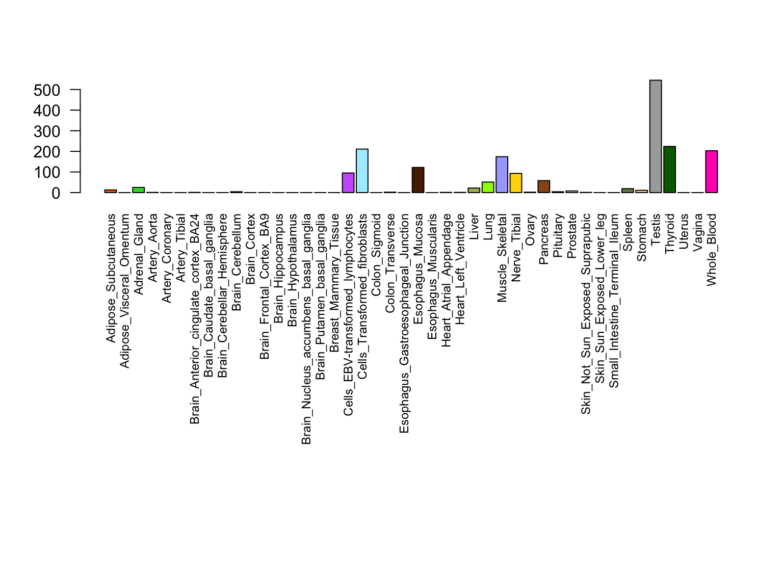
Expand here to see past versions of plot-counts-1.png:
| Version | Author | Date |
|---|---|---|
| df200f8 | Peter Carbonetto | 2018-06-06 |
Testis stands out as the tissue with the most tissue-specific effects. Other tissues showing stronger-than-average tissue specificity include skeletal muscle, thyroid and transformed cell lines (fibroblasts and LCLs).
Session information
sessionInfo()
# R version 3.4.3 (2017-11-30)
# Platform: x86_64-apple-darwin15.6.0 (64-bit)
# Running under: macOS High Sierra 10.13.5
#
# Matrix products: default
# BLAS: /Library/Frameworks/R.framework/Versions/3.4/Resources/lib/libRblas.0.dylib
# LAPACK: /Library/Frameworks/R.framework/Versions/3.4/Resources/lib/libRlapack.dylib
#
# locale:
# [1] en_US.UTF-8/en_US.UTF-8/en_US.UTF-8/C/en_US.UTF-8/en_US.UTF-8
#
# attached base packages:
# [1] stats     graphics  grDevices utils     datasets  methods   base
#
# loaded via a namespace (and not attached):
#  [1] workflowr_1.0.1.9000 Rcpp_0.12.17         digest_0.6.15
#  [4] rprojroot_1.3-2      R.methodsS3_1.7.1    backports_1.1.2
#  [7] git2r_0.21.0         magrittr_1.5         evaluate_0.10.1
# [10] stringi_1.1.7        whisker_0.3-2        R.oo_1.21.0
# [13] R.utils_2.6.0        rmarkdown_1.9        tools_3.4.3
# [16] stringr_1.3.0        yaml_2.1.18          compiler_3.4.3
# [19] htmltools_0.3.6      knitr_1.20
This reproducible R Markdown analysis was created with workflowr 1.0.1.9000