Crop-seq Workflow
Alan Selewa
Last updated: 2018-11-20
workflowr checks: (Click a bullet for more information)-
✔ R Markdown file: up-to-date
Great! Since the R Markdown file has been committed to the Git repository, you know the exact version of the code that produced these results.
-
✔ Environment: empty
Great job! The global environment was empty. Objects defined in the global environment can affect the analysis in your R Markdown file in unknown ways. For reproduciblity it’s best to always run the code in an empty environment.
-
✔ Seed:
set.seed(20181119)The command
set.seed(20181119)was run prior to running the code in the R Markdown file. Setting a seed ensures that any results that rely on randomness, e.g. subsampling or permutations, are reproducible. -
✔ Session information: recorded
Great job! Recording the operating system, R version, and package versions is critical for reproducibility.
-
Great! You are using Git for version control. Tracking code development and connecting the code version to the results is critical for reproducibility. The version displayed above was the version of the Git repository at the time these results were generated.✔ Repository version: 8be64d0
Note that you need to be careful to ensure that all relevant files for the analysis have been committed to Git prior to generating the results (you can usewflow_publishorwflow_git_commit). workflowr only checks the R Markdown file, but you know if there are other scripts or data files that it depends on. Below is the status of the Git repository when the results were generated:
Note that any generated files, e.g. HTML, png, CSS, etc., are not included in this status report because it is ok for generated content to have uncommitted changes.Ignored files: Ignored: .DS_Store Ignored: .Rproj.user/ Ignored: analysis/figure/ Ignored: data/.DS_Store Ignored: docs/figure/ Untracked files: Untracked: data/CROP_data_from_Alan/ Untracked: data/Gmail - Fw_ CROP-seq analysis.pdf Untracked: data/cell_ranger_from_Alan/ Untracked: data/data_from_Siwei/ Unstaged changes: Modified: README.md
Expand here to see past versions:
| File | Version | Author | Date | Message |
|---|---|---|---|---|
| Rmd | 8be64d0 | simingz | 2018-11-20 | First |
Preprocessing
I assume the following files are in the working directory
- NSC0507 - raw fastq
- NSC08 - raw fastq
- reference - spiked reference genome and annotations
Load CellRanger and check version
module load cellranger
which cellranger
My version is 2.1.1
We need to first make a special reference file for CellRanger. It uses the spiked reference genome and spiked GTF file
cd reference/
cellranger mkref --nthreads=1
                 --genome=cellranger_ref
                 --fasta=hg38_gRNA_spiked_11Jun2018.fa
                 --genes=gencode_gRNA_spiked_filtered_11Jul2018.gtf
cd ..
Now we are ready to make our count matrix. We run cellranger count on both datasets. I expect 2000 cells based on what the experimentalists told me. These commands will use all available cores.
cellranger count --id=NSC0507_CR
                 --transcriptome=reference/cellranger_ref
                 --fastqs=NSC0507//fastq/
                 --expect-cells=2000

cellranger count --id=NSC08_CR
                 --transcriptome=reference/cellranger_ref
                 --fastqs=NSC08/fastq/
                 --expect-cells=2000
This command will generateo two new cellranger directories with the id as the filename. The output details can be found at the bottom of this page. The keu file is the filtered_gene_bc_matrices.h5. The filtered here means that only cells with detected barcodes are included.
Unfortunately, all of matrices are in either MEX or HDF5 format. We can use the following command to get a CSV file:
cellranger mat2csv NSC0507_CR/outs/filtered_gene_bc_matrices_h5.h5 NSC0507.csv

cellranger mat2csv NSC08_CR/outs/filtered_gene_bc_matrices_h5.h5 NSC08.csv
Exploratory data analysis
I assume that the following are in the parent directory:
- NSC08.csv
- NSC0507.csv
- gRNAs.txt
Now we have the count matrices and we can move on to R.
library(data.table)

nsc0507 <- data.frame(fread('data/cell_ranger_from_Alan/NSC0507.csv',sep=','),row.names=1)
Read 33.4% of 29922 rows
Read 29922 rows and 2100 (of 2100) columns from 0.119 GB file in 00:00:04
colnames(nsc0507) = paste(colnames(nsc0507),'0507') #prevent overlapping barcodes
nsc08 <- data.frame(fread('data/cell_ranger_from_Alan/NSC08.csv',sep=','),row.names=1)
Read 66.8% of 29922 rows
Read 29922 rows and 2101 (of 2101) columns from 0.119 GB file in 00:00:04
colnames(nsc08) = paste(colnames(nsc08),'08') #prevent overlapping barcodesCombine into one matrix and remove genes found
comb = cbind(nsc08, nsc0507)Load list of guide RNAs and subset the combined expression matrix
gRNAs = readLines('data/CROP_data_from_Alan/gRNAs.txt')
gRNA.dge = comb[gRNAs,]
Frequency distribution of guide RNAs:
barplot(table(colSums(gRNA.dge>0)),xlab='Number of Guide RNAs',ylab='Number of Cells')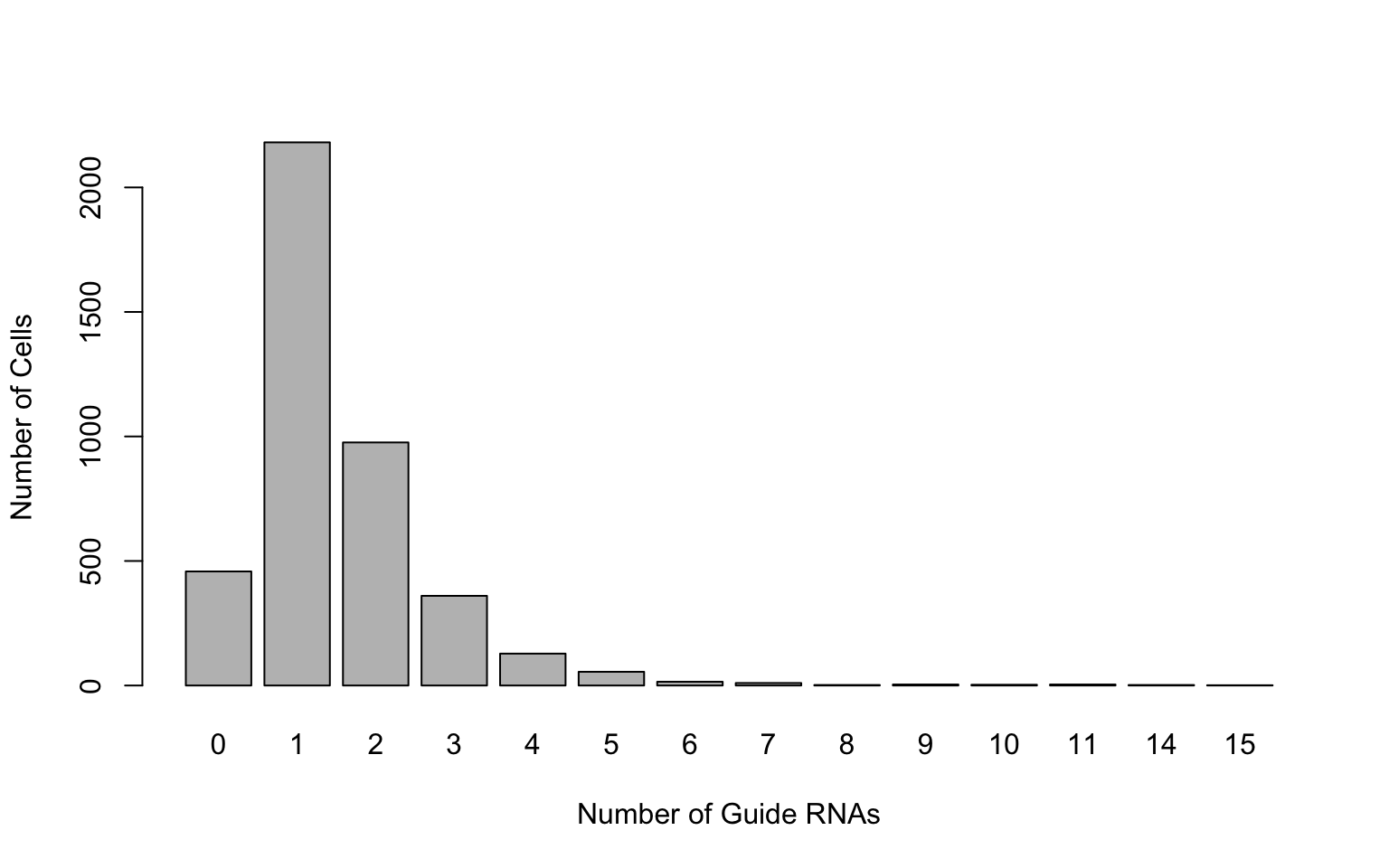
We would like to collapse expression data of guide RNAs from the same locus.
library(dplyr)

gRNA.dge$label = sapply(strsplit(gRNAs,split = '_'), function(x){x[1]})
gRNA.dge.col = as.data.frame(gRNA.dge %>% group_by(label) %>% summarise_all(funs(sum)))
row.names(gRNA.dge.col) = gRNA.dge.col$label
gRNAs.col = rownames(gRNA.dge.col)
gRNA.dge.col$label = NULL

#Controls (cells without any gRNAs)
ctrls = colnames(comb)[which(colSums(gRNA.dge.col)==0)]

#Singletons (cells with only 1 gRNA)
singles = colnames(comb)[which(colSums(gRNA.dge.col>0)==1)]

grna.det.rate = rowSums(gRNA.dge.col[,singles]>0)
order.grna = gRNAs.col[order(grna.det.rate,decreasing = T)]

grna.det.df = data.frame(det=grna.det.rate, gRNAs=factor(gRNAs.col, levels = order.grna))

library(ggplot2)
ggplot(grna.det.df, aes(x=gRNAs, y=det)) + geom_bar(stat="identity") + theme(axis.text.x = element_text(angle = 90, hjust = 1)) +
  xlab('guide RNAs') + ylab('Number of Cells')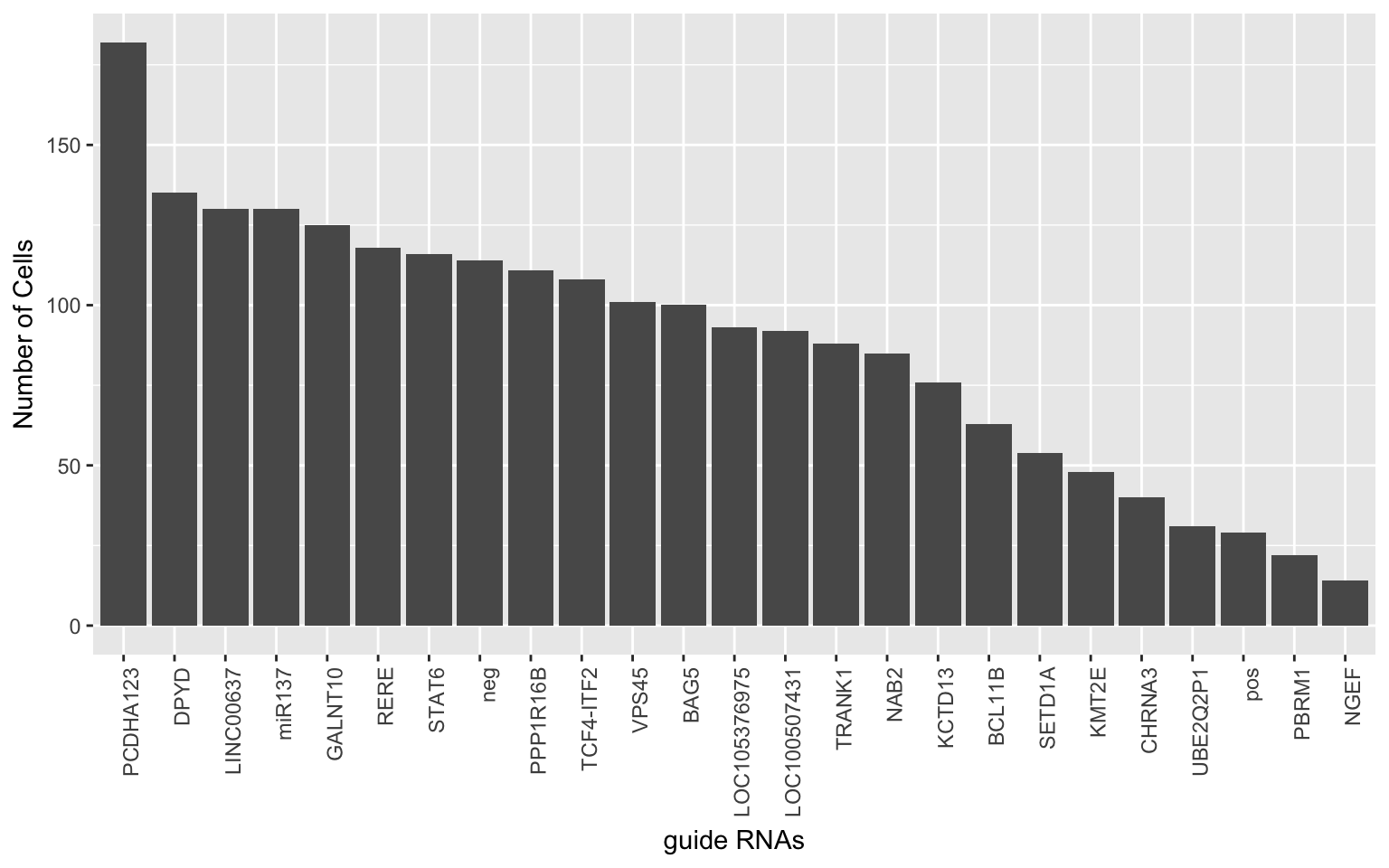
Differential Expression analysis
This paper shows that DESeq2 has one of the lowest false positive rates for UMI data. We use this to perform our differential expression analysis.
Install DESeq2
source("https://bioconductor.org/biocLite.R")
biocLite("DESeq2")
We use DESeq2 on cells that have/dont have the top guide RNA, which is VPS45_2
library(DESeq2)

g = order.grna[1]
g.only.cells = singles[which(gRNA.dge[g,singles] > 0)]

#We only test the expression among the top expressed genes
comb.filt = comb[rowSums(comb>0)>1000,]

sampleType = factor(c(rep('G',length(g.only.cells)),rep('N',length(ctrls))),levels = c('N','G'))

dds = DESeqDataSetFromMatrix(countData = comb.filt[,c(g.only.cells, ctrls)],
                             colData = data.frame(row.names = c(g.only.cells, ctrls), sampleType=sampleType),
                             design = ~sampleType) # we're testing for the different condidtions

dds = estimateSizeFactors(dds)

dds = DESeq(dds)
res = results(dds)

# At FDR of 10%
resSig <- subset(res, padj < 0.1)
dim(resSig)[1]

write.table(resSig,paste(g,'_DESeq2_FD10.1.txt'),sep='\t',quote=F,row.names = T,col.names = T)

upReg = resSig[resSig$log2FoldChange>0,]
downReg = resSig[resSig$log2FoldChange<0,]

mean(upReg$log2FoldChange)
mean(downReg$log2FoldChange)
I set eval=FALSE above because it can take several minutes to perform the expression analysis.
Session information
sessionInfo()R version 3.3.2 (2016-10-31)
Platform: x86_64-apple-darwin11.4.2 (64-bit)
Running under: OS X El Capitan 10.11.6
locale:
[1] en_US.UTF-8/en_US.UTF-8/en_US.UTF-8/C/en_US.UTF-8/en_US.UTF-8
attached base packages:
[1] stats graphics grDevices utils datasets methods base
other attached packages:
[1] ggplot2_2.2.1 dplyr_0.7.5 data.table_1.10.4
loaded via a namespace (and not attached):
[1] Rcpp_0.12.17 knitr_1.20 bindr_0.1.1
[4] whisker_0.3-2 magrittr_1.5 workflowr_1.1.1
[7] munsell_0.4.3 tidyselect_0.2.4 colorspace_1.3-1
[10] R6_2.2.2 rlang_0.2.1 plyr_1.8.4
[13] stringr_1.2.0 tools_3.3.2 grid_3.3.2
[16] gtable_0.2.0 R.oo_1.22.0 git2r_0.18.0
[19] htmltools_0.3.6 lazyeval_0.2.0 yaml_2.1.16
[22] rprojroot_1.2 digest_0.6.12 assertthat_0.2.0
[25] tibble_1.4.2 bindrcpp_0.2.2 purrr_0.2.5
[28] R.utils_2.7.0 glue_1.2.0 evaluate_0.10
[31] rmarkdown_1.10 labeling_0.3 stringi_1.1.5
[34] pillar_1.2.3 scales_0.5.0 backports_1.0.5
[37] R.methodsS3_1.7.1 pkgconfig_2.0.1 This reproducible R Markdown analysis was created with workflowr 1.1.1