Assessing the effects of long-term trends
Robert W Schlegel
2019-03-19
Last updated: 2019-03-19
workflowr checks: (Click a bullet for more information)-
✔ R Markdown file: up-to-date
Great! Since the R Markdown file has been committed to the Git repository, you know the exact version of the code that produced these results.
-
✔ Environment: empty
Great job! The global environment was empty. Objects defined in the global environment can affect the analysis in your R Markdown file in unknown ways. For reproduciblity it’s best to always run the code in an empty environment.
-
✔ Seed:
set.seed(20190319)The command
set.seed(20190319)was run prior to running the code in the R Markdown file. Setting a seed ensures that any results that rely on randomness, e.g. subsampling or permutations, are reproducible. -
✔ Session information: recorded
Great job! Recording the operating system, R version, and package versions is critical for reproducibility.
-
Great! You are using Git for version control. Tracking code development and connecting the code version to the results is critical for reproducibility. The version displayed above was the version of the Git repository at the time these results were generated.✔ Repository version: 64ac134
Note that you need to be careful to ensure that all relevant files for the analysis have been committed to Git prior to generating the results (you can usewflow_publishorwflow_git_commit). workflowr only checks the R Markdown file, but you know if there are other scripts or data files that it depends on. Below is the status of the Git repository when the results were generated:
Note that any generated files, e.g. HTML, png, CSS, etc., are not included in this status report because it is ok for generated content to have uncommitted changes.Ignored files: Ignored: .Rhistory Ignored: .Rproj.user/ Ignored: vignettes/data/sst_ALL_clim_only.Rdata Ignored: vignettes/data/sst_ALL_event_aov_tukey.Rdata Ignored: vignettes/data/sst_ALL_flat.Rdata Ignored: vignettes/data/sst_ALL_miss.Rdata Ignored: vignettes/data/sst_ALL_miss_cat_chi.Rdata Ignored: vignettes/data/sst_ALL_miss_clim_event_cat.Rdata Ignored: vignettes/data/sst_ALL_miss_clim_only.Rdata Ignored: vignettes/data/sst_ALL_repl.Rdata Ignored: vignettes/data/sst_ALL_smooth.Rdata Ignored: vignettes/data/sst_ALL_smooth_aov_tukey.Rdata Ignored: vignettes/data/sst_ALL_smooth_event.Rdata Ignored: vignettes/data/sst_ALL_trend.Rdata Ignored: vignettes/data/sst_ALL_trend_clim_event_cat.Rdata Untracked files: Untracked: analysis/bibliography.bib Untracked: analysis/data/ Untracked: code/functions.R Untracked: code/workflow.R Untracked: data/sst_WA.csv Untracked: docs/figure/ Unstaged changes: Modified: NEWS.md
Expand here to see past versions:
| File | Version | Author | Date | Message |
|---|---|---|---|---|
| Rmd | 64ac134 | robwschlegel | 2019-03-19 | Publish analysis files |
Overview
The last major variable we want to look at that could potentially affect accurate MHW detection is the long-term (secular) trend present in a time series. To do so we will be using the same de-trended data from the previous two vignettes and slowly adding in decadal trends from 0.01 to 0.30 °C/dec in 0.0.1 °C/dec steps.
library(tidyverse)
library(broom)
library(heatwaveR, lib.loc = "~/R-packages/")
# cat(paste0("heatwaveR version = ",packageDescription("heatwaveR")$Version))
library(lubridate) # This is intentionally activated after data.table
library(fasttime)
library(ggpubr)
library(boot)
library(FNN)
library(mgcv)
# library(padr)
library(ggridges)
Trending
The following chunks contain the code used to systematically add increasing decadal trends to the three reference time series.
# First load the de-trended re-sampled data created in the duration vignette
load("data/sst_ALL_flat.Rdata")

# Function for adding trends to data
# rate <- 0.1
add_trend <- function(rate){
  daily_step <- rate/3652.5
  res <- sst_ALL_detrend %>%
    group_by(site, rep) %>%
    mutate(row_index = 1:n(),
           temp = temp + (row_index*daily_step)) %>%
    mutate(trend = as.character(rate)) %>%
    select(-row_index)
  return(res)
}

# Add the trends and save
doMC::registerDoMC(cores = 50)
sst_ALL_trend <- plyr::ldply(seq(0.00, 0.30, 0.01), add_trend, .parallel = T)
save(sst_ALL_trend, file = "data/sst_ALL_trend.Rdata")
Climatology statistics
# This file is not uploaded to GitHub as it is too large
# One must first run the above code locally to generate and save the file
load("data/sst_ALL_trend.Rdata")

# Calculate climatologies, events, and categories on shrinking time series
clim_event_cat_calc <- function(df){
  res <- df %>%
    nest() %>%
    mutate(clims = map(data, ts2clm,
                       climatologyPeriod = c("1982-01-01", "2011-12-31")),
           events = map(clims, detect_event),
           cats = map(events, category)) %>%
    select(-data, -clims)
  return(res)
}

# Calculate all of the MHW related results
doMC::registerDoMC(cores = 50)
sst_ALL_trend_clim_event_cat <- plyr::ddply(sst_ALL_trend, c("trend", "site"),
                                           clim_event_cat_calc, .parallel = T)
save(sst_ALL_trend_clim_event_cat, file = "data/sst_ALL_trend_clim_event_cat.Rdata")
# This file is not uploaded to GitHub as it is too large
# One must first run the above code locally to generate and save the file
load("data/sst_ALL_trend_clim_event_cat.Rdata")
# Wrapper function to speed up the extraction of clims
trend_clim_only <- function(df){
res <- df %>%
select(-cats) %>%
unnest(events) %>%
filter(row_number() %% 2 == 1) %>%
unnest(events) %>%
select(trend:doy, seas:thresh) %>%
unique() %>%
arrange(doy)
}
# Pull out only seas and thresh for ease of plotting
doMC::registerDoMC(cores = 50)
sst_ALL_trend_clim_only <- plyr::ddply(sst_ALL_trend_clim_event_cat, c("trend", "site"),
trend_clim_only, .parallel = T)
save(sst_ALL_trend_clim_only, file = "data/sst_ALL_trend_clim_only.Rdata")load("~/MHWdetection/analysis/data/sst_ALL_trend_clim_only.Rdata")ggplot(sst_ALL_trend_clim_only,
aes(y = seas, x = doy, colour = as.numeric(trend))) +
geom_line(alpha = 0.3, aes(group = trend)) +
scale_colour_viridis_c() +
facet_wrap(~site, ncol = 1, scales = "free_y") +
labs(x = "Calendar day of year", y = "Temp. (°C)", colour = "trend (°C/dec)")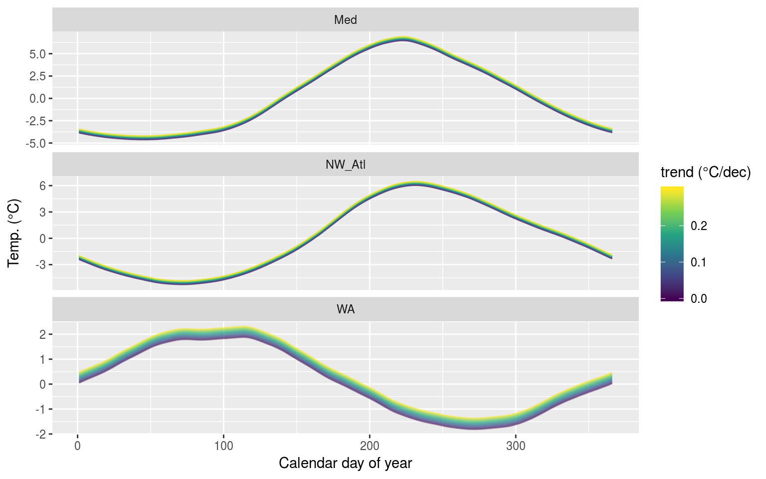
The seasonal signals created from time series with increasingly large decadal trends added.
Looking at the range of seasonal signals we see how pronounced the effect of adding a decadal trend is to WA over the other two time series. This is because the proportionate to the overall range of the seasonal signal, we are adding much more to the WA time series than the others.
ggplot(sst_ALL_trend_clim_only,
       aes(y = thresh, x = doy, colour = as.numeric(trend))) +
  geom_line(alpha = 0.3, aes(group = trend)) +
  scale_colour_viridis_c() +
  facet_wrap(~site, ncol = 1, scales = "free_y") +
  labs(x = "Calendar day of year", y = "Temp. (°C)", colour = "trend (°C/dec)")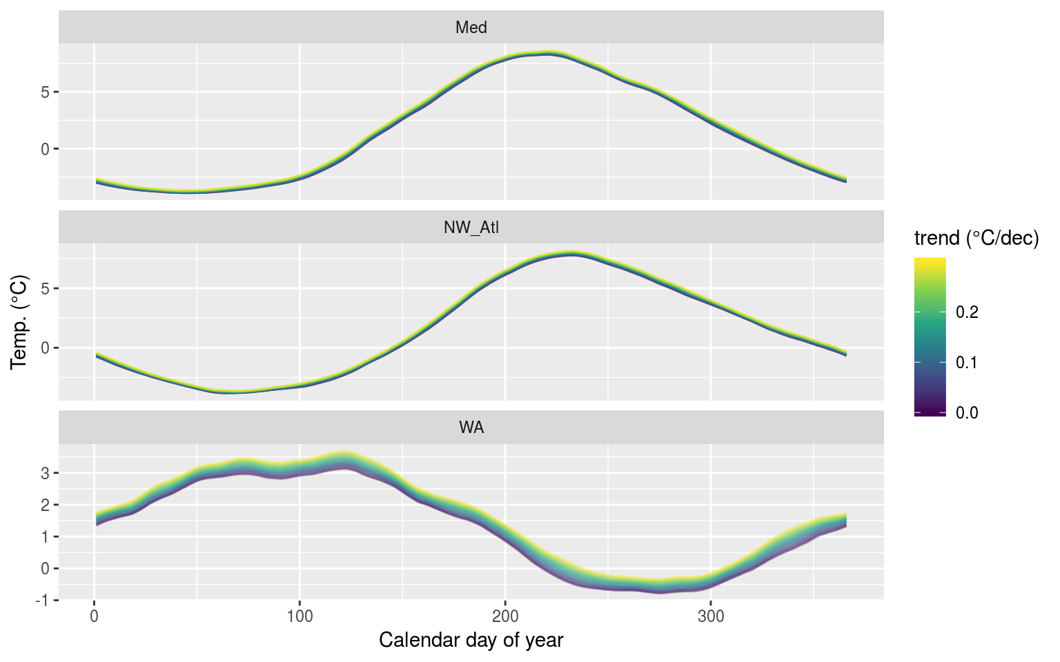
The 90th percentile thresholds created from time series with increasingly large decadal trends added.
Interestingly the increase in the 90th percentile threshold appears to be similar for the 90th percentile threshold as it is for the seasonal signal. This implies that the upcoming results are likely to vary from the previous two vignettes.
ANOVA p-values
Given that there are perceptible differences in the seasonal signals as decadal trends increase, an ANOVA will almost certainly determine these differences to be significant.
# Run an ANOVA on each metric of the event results from
# the same amount of trending data and get the p-value
aov_p <- function(df){
  aov_models <- df[ , -grep("trend", names(df))] %>%
    map(~ aov(.x ~ df$trend)) %>%
    map_dfr(~ broom::tidy(.), .id = 'metric') %>%
    mutate(p.value = round(p.value, 4)) %>%
    filter(term != "Residuals") %>%
    select(metric, p.value)
  return(aov_models)
  }

# Run an ANOVA on each metric and then a Tukey test
aov_tukey <- function(df){
  aov_tukey <- df[ , -grep("trend", names(df))] %>%
    map(~ TukeyHSD(aov(.x ~ df$trend))) %>%
    map_dfr(~ broom::tidy(.), .id = 'metric') %>%
    mutate(p.value = round(adj.p.value, 4)) %>%
    # filter(term != "Residuals") %>%
    select(metric, comparison, adj.p.value) %>%
    # filter(adj.p.value <= 0.05) %>%
    arrange(metric, adj.p.value)
  return(aov_tukey)
}

# Quick wrapper for getting results for ANOVA and Tukey on clims
# df <- sst_ALL_trend_clim_only %>%
#   filter(site == "WA") %>%
#   select(-site)
clim_aov_tukey <- function(df){
  res <- df %>%
    # filter(trend != "0.00") %>%
    select(trend, seas, thresh) %>%
    mutate(trend = as.factor(trend)) %>%
    nest() %>%
    mutate(aov = map(data, aov_p),
           tukey = map(data, aov_tukey)) %>%
    select(-data)
  return(res)
}
# This file is not uploaded to GitHub as it is too large
# One must first run the above code locally to generate and save the file
load("data/sst_ALL_trend_clim_only.Rdata")
doMC::registerDoMC(cores = 50)
sst_ALL_trend_clim_aov_tukey <- plyr::ddply(sst_ALL_trend_clim_only, c("site"),
clim_aov_tukey, .parallel = T)
save(sst_ALL_trend_clim_aov_tukey, file = "data/sst_ALL_trend_clim_aov_tukey.Rdata")
# rm(sst_ALL_smooth, sst_ALL_smooth_aov_tukey)load("~/MHWdetection/analysis/data/sst_ALL_trend_clim_aov_tukey.Rdata")
sst_ALL_trend_clim_aov <- sst_ALL_trend_clim_aov_tukey %>%
select(-tukey) %>%
unnest()
ggplot(sst_ALL_trend_clim_aov, aes(x = site, y = metric)) +
geom_tile(aes(fill = p.value)) +
geom_text(aes(label = round(p.value, 2))) +
scale_fill_gradient2(midpoint = 0.1)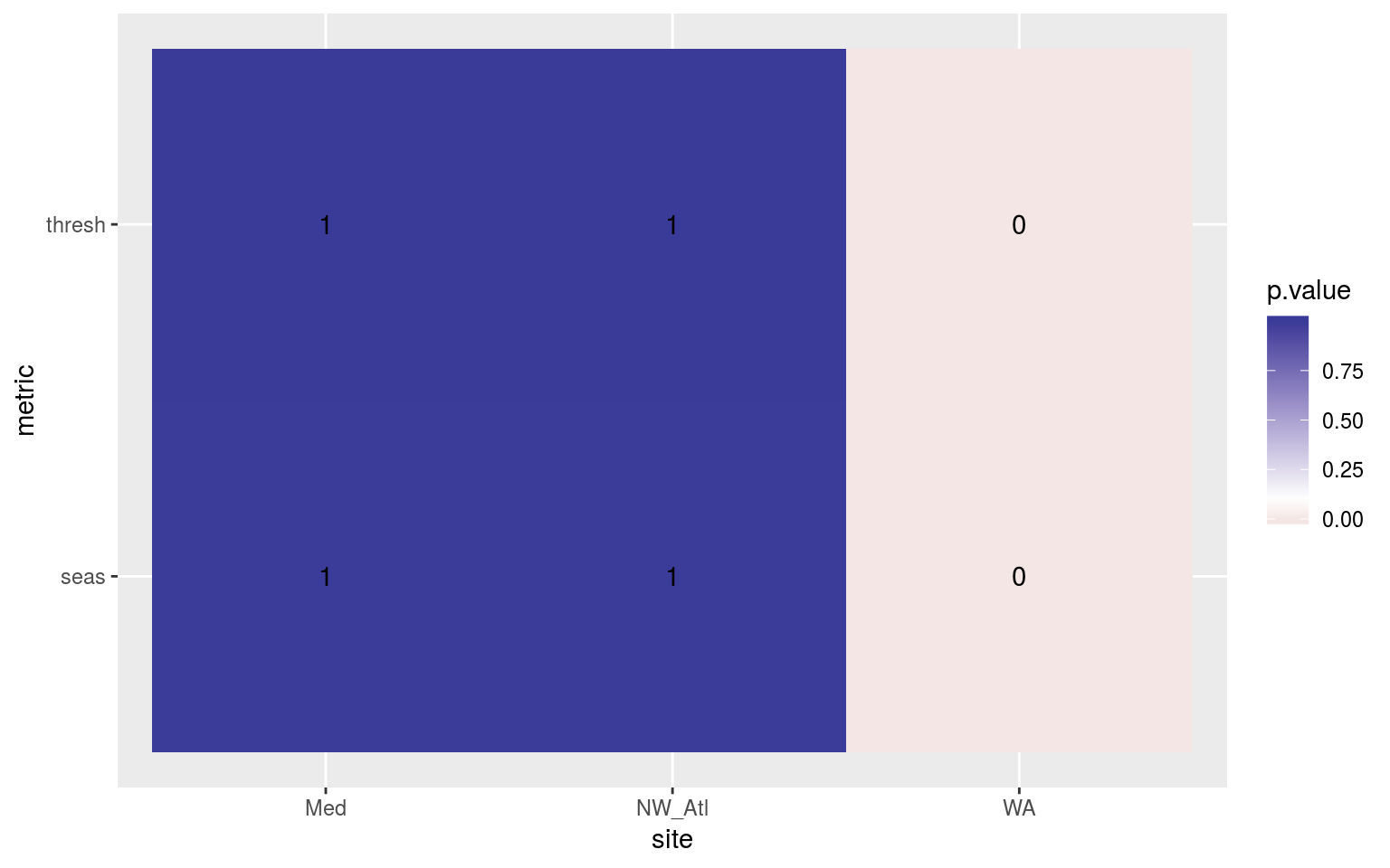
Heatmap showing the ANOVA results for the comparisons of the clim values for the different proportions of trending data. The 90th percentile thresholds are significantly different at p < 0.05 but the seasonal signals are not.
We may see in the figure above that the climatologies do not differ appreciably across all of the decadal trends used for the Med and NW_Atl. The climatologies do however differ significantly for the WA time series.
Post-hoc Tukey test
And now to see where exactly the WA climatologies begin to diverge.
sst_ALL_trend_clim_tukey <- sst_ALL_trend_clim_aov_tukey %>%
  select(-aov) %>%
  unnest()

# Create a summary for better plotting
clim_tukey_summary <- sst_ALL_trend_clim_tukey %>%
  separate(comparison, into = c("comp_left", "comp_right"), sep = "-") %>%
  mutate(comp_left = as.numeric(comp_left),
         comp_right = as.numeric(comp_right)) %>%
  filter(comp_left == 0 | comp_right == 0) %>%
  mutate(comp_dif = abs(round(comp_right - comp_left, 2))) %>%
  filter(adj.p.value <= 0.05) %>%
  group_by(site, metric, comp_dif)

ggplot(clim_tukey_summary, aes(x = comp_dif, y = site)) +
  geom_line() +
  geom_point(size = 0.5) +
  facet_wrap(~metric, ncol = 1) +
  scale_x_continuous(limits = c(0, 0.3)) +
  labs(x = "Trend (°C/dec)", y = NULL,
       colour = "Sig. dif.\nout of 100")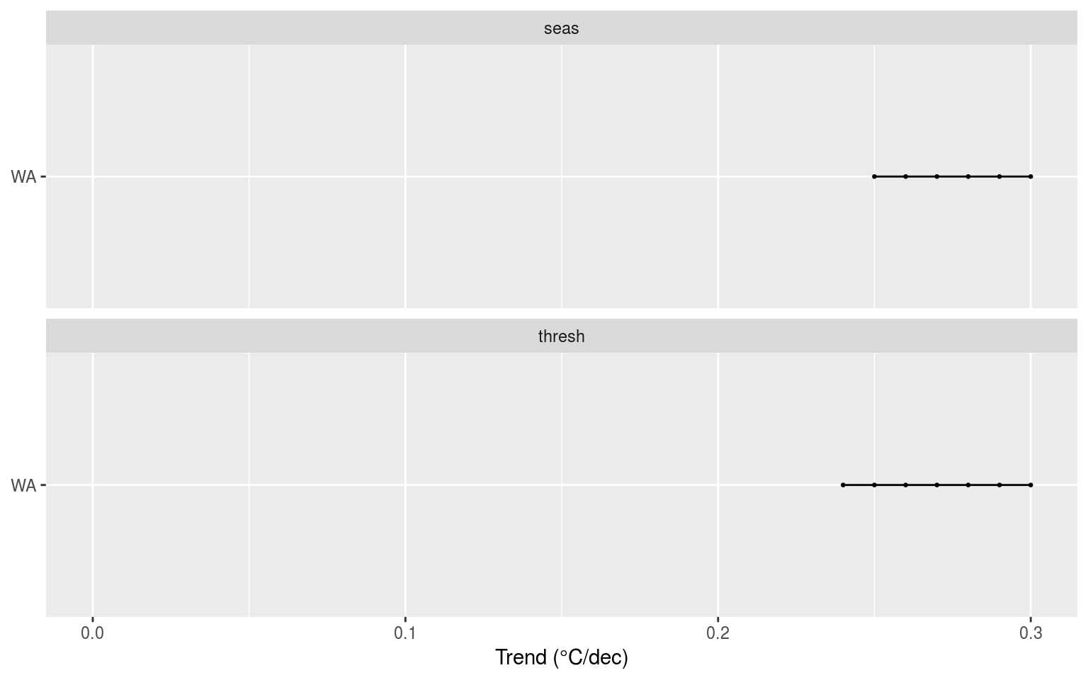
Segments showing the range of decadal trends added to the data when climatologies were significantly different.
In the figure above we see that the WA seasonal signals become significantly different at a decadal trend of 0.25°C/dec, and the 90th percentile threshold becomes sig. dif. at 0.24°C/dec.
Kolmogorov-Smirnov tests
Now knowing that the daily values that make up the climatologies tend to differ based on the decadal trend added, as seen with the ANOVA and Tukey results, we want to check where the distributions of the climatologies themselves begin to differ. We will do this through a series of pair-wise two-sample KS tests.
# Extract the true climatologies
sst_ALL_trend_clim_only_0 <- sst_ALL_trend_clim_only %>%
  filter(trend == 0)

# KS function
# Takes one rep of trending data and compares it against the complete signal
clim_KS_p <- function(df){
  df_comp <- sst_ALL_trend_clim_only_0 %>%
    filter(site == df$site[1])
  res <- data.frame(site = df$site[1],
                    seas = round(ks.test(df$seas, df_comp$seas)$p.value, 4),
                    thresh = round(ks.test(df$thresh, df_comp$thresh)$p.value, 4))
  return(res)
}

# The KS results
suppressWarnings( # Suppress perfect match warnings
sst_ALL_trend_clim_KS_p <- sst_ALL_trend_clim_only %>%
  filter(trend != 0) %>%
  mutate(trend = as.factor(trend)) %>%
  mutate(site2 = site) %>%
  group_by(site2, trend) %>%
  nest() %>%
  mutate(res = map(data, clim_KS_p)) %>%
  select(-data) %>%
  unnest() %>%
  select(site, trend, seas, thresh) %>%
  gather(key = metric, value = p.value, -site, - trend)
)
save(sst_ALL_trend_clim_KS_p, file = "data/sst_ALL_trend_clim_KS_p.Rdata")
load("~/MHWdetection/analysis/data/sst_ALL_trend_clim_KS_p.Rdata")
# Filter non-significant results
KS_sig <- sst_ALL_trend_clim_KS_p %>%
filter(p.value <= 0.05) %>%
group_by(site, trend, metric) %>%
summarise(count = n()) %>%
ungroup()
# Manually pad in NA for trending percentages with no significant differences
# KS_sig <- rbind(KS_sig, data.frame(site = "Med", metric = "thresh", perc = 100:74, count = NA))
# KS_sig <- rbind(KS_sig, data.frame(site = "NW_Atl", metric = "thresh", perc = 100:79, count = NA))
# KS_sig <- rbind(KS_sig, data.frame(site = "WA", metric = "thresh", perc = 100:92, count = NA))
ggplot(KS_sig, aes(x = as.numeric(trend), y = site)) +
geom_line(aes(group = site)) +
geom_point() +
facet_wrap(~metric, ncol = 1) +
# scale_x_reverse(breaks = seq(5, 35, 5)) +
labs(x = "Added decadal trend (°C)", y = NULL)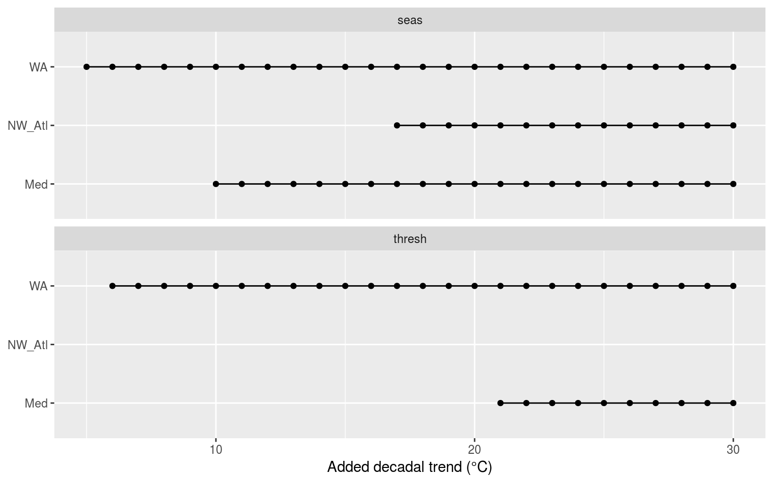
Dot and line plot showing the p-value results from KS tests comparing the climatology statistics for increasingly large decadal trends against the de-trended climatologies for each of the three reference time series.
Surprisingly the above figure shows that the seasonal signal is much more sensitive than the 90th percentile threshold to the addition of decadal trends. The WA time series remains the most sensitive with sig. dif. occurring at an added decadal trend of 0.05°C. The interesting thing here is that the NW_Atl threshold never had a significantly different distribution regardless of the amount added.
Thinking about this more I have alighted upon the idea that because the threshold is determined by the largest values detected on any given calendar day, the size of the deadal trend present in the data could be deminished by the fact that some of the values creating the threshold will be from the earlier portion of the time series before the decadal trend realy starts having an effect.
MHW metrics
ANOVA
# Quick wrapper for getting results for ANOVA and Tukey on event metrics
# df <- sst_ALL_trend_clim_event_cat %>%
#   filter(site == "WA") %>%
#   select(-site)
event_aov_tukey <- function(df){
  res <- df %>%
    select(-cats) %>%
    unnest(events) %>%
    filter(row_number() %% 2 == 0) %>%
    unnest(events) %>%
    # select(trend) %>%
    # filter(trend != "0.00") %>%
    select(trend, duration, intensity_mean, intensity_max, intensity_cumulative) %>%
    mutate(trend = as.factor(trend)) %>%
    nest() %>%
    mutate(aov = map(data, aov_p),
           tukey = map(data, aov_tukey)) %>%
    select(-data)
  return(res)
}

# This file is not uploaded to GitHub as it is too large
# One must first run the above code locally to generate and save the file
load("data/sst_ALL_trend_clim_event_cat.Rdata")
doMC::registerDoMC(cores = 50)
sst_ALL_trend_event_aov_tukey <- plyr::ddply(sst_ALL_trend_clim_event_cat, c("site"),
                                             event_aov_tukey, .parallel = T)
save(sst_ALL_trend_event_aov_tukey, file = "data/sst_ALL_trend_event_aov_tukey.Rdata")
# rm(sst_ALL_smooth, sst_ALL_smooth_aov_tukey)
load("~/MHWdetection/analysis/data/sst_ALL_trend_event_aov_tukey.Rdata")
# ANOVA p
sst_ALL_trend_event_aov_p <- sst_ALL_trend_event_aov_tukey %>%
select(-tukey) %>%
unnest()
event_aov_plot <- sst_ALL_trend_event_aov_p %>%
group_by(site, metric) %>%
filter(p.value <= 0.05) %>%
summarise(count = n())
# visualise
# ggplot(event_aov_plot, aes(x = site, y = metric)) +
# geom_tile(aes(fill = count)) +
# geom_text(aes(label = count)) +
# scale_fill_viridis_c() +
# theme(axis.text.y = element_text(angle = 90, hjust = 0.5))There is no figure here because there is nothing to show. None of the metrics for any of the time series were significantly different.
Post-hoc Tukey test
sst_ALL_trend_event_tukey <- sst_ALL_trend_event_aov_tukey %>%
  select(-aov) %>%
  unnest()

# Create a summary for better plotting
event_tukey_summary <- sst_ALL_trend_event_tukey %>%
  separate(comparison, into = c("comp_left", "comp_right"), sep = "-") %>%
  mutate(comp_left = as.numeric(comp_left),
         comp_right = as.numeric(comp_right)) %>%
  filter(comp_left == 0 | comp_right == 0) %>%
  mutate(comp_dif = abs(round(comp_right - comp_left, 2))) %>%
  filter(adj.p.value <= 0.05) %>%
  group_by(site, metric, comp_dif)

# ggplot(event_tukey_summary, aes(x = comp_dif, y = site)) +
#   geom_line(aes(colour = count)) +
#   geom_point(aes(colour = count), size = 0.5) +
#   facet_wrap(~metric, ncol = 1) +
#   scale_colour_viridis_c() +
#   # scale_x_reverse(breaks = seq(5, 35, 5)) +
#   labs(x = "trending data (%)", y = NULL,
#        colour = "Sig. dif.\nout of 100")
Nope, no differences on a pair-wise basis. How could there be when the ANOVAs weren’t significant.
Confidence intervals
# Calculate CIs using a bootstrapping technique to deal with the non-normal small sample sizes

# df <- sst_ALL_both_event %>%
#   filter(lubridate::year(date_peak) >= 2012,
#          site == "WA",
#          trend == "detrended") %>%
#   select(year_index, duration, intensity_mean, intensity_max, intensity_cumulative) #%>%
  # select(site, trend, year_index, duration, intensity_mean, intensity_max, intensity_cumulative) #%>%
  # nest(-site, -trend)
Bmean <- function(data, indices) {
  d <- data[indices] # allows boot to select sample
    return(mean(d))
}

event_CI <- function(df){
  df_conf <- gather(df, key = "metric", value = "value") %>%
    group_by(metric) %>%
    # ggplot(aes(x = value)) +
    # geom_histogram(aes(fill = metric)) +
    # facet_wrap(~metric, scales = "free_x")
    summarise(lower = boot.ci(boot(data=value, statistic=Bmean, R=1000), type = "basic")$basic[4],
              mid = mean(value),
              upper = boot.ci(boot(data=value, statistic=Bmean, R=1000), type = "basic")$basic[5],
              n = n()) %>%
    mutate_if(is.numeric, round, 4)
  return(df_conf)
}

sst_ALL_trend_event_CI <- sst_ALL_trend_clim_event_cat %>%
  select(-cats) %>%
  unnest(events) %>%
  filter(row_number() %% 2 == 0) %>%
  unnest(events) %>%
  select(site, trend, duration, intensity_mean, intensity_max, intensity_cumulative) %>%
  nest(-site, -trend) %>%
  mutate(res = map(data, event_CI)) %>%
  select(-data) %>%
  unnest()

save(sst_ALL_trend_event_CI, file = "data/sst_ALL_trend_event_CI.Rdata")
load("~/MHWdetection/analysis/data/sst_ALL_trend_event_CI.Rdata")
ggplot(sst_ALL_trend_event_CI, aes(x = trend)) +
geom_errorbar(width = 1, alpha = 0.8,
aes(ymin = lower, ymax = upper)) +
# geom_text(aes(label = n, y = upper*1.3, colour = trend), size = 3) +
geom_point(aes(y = mid), size = 1, alpha = 0.7) +
facet_grid(metric~site, scales = "free_y") +
labs(x = "Trend (°C)", y = NULL)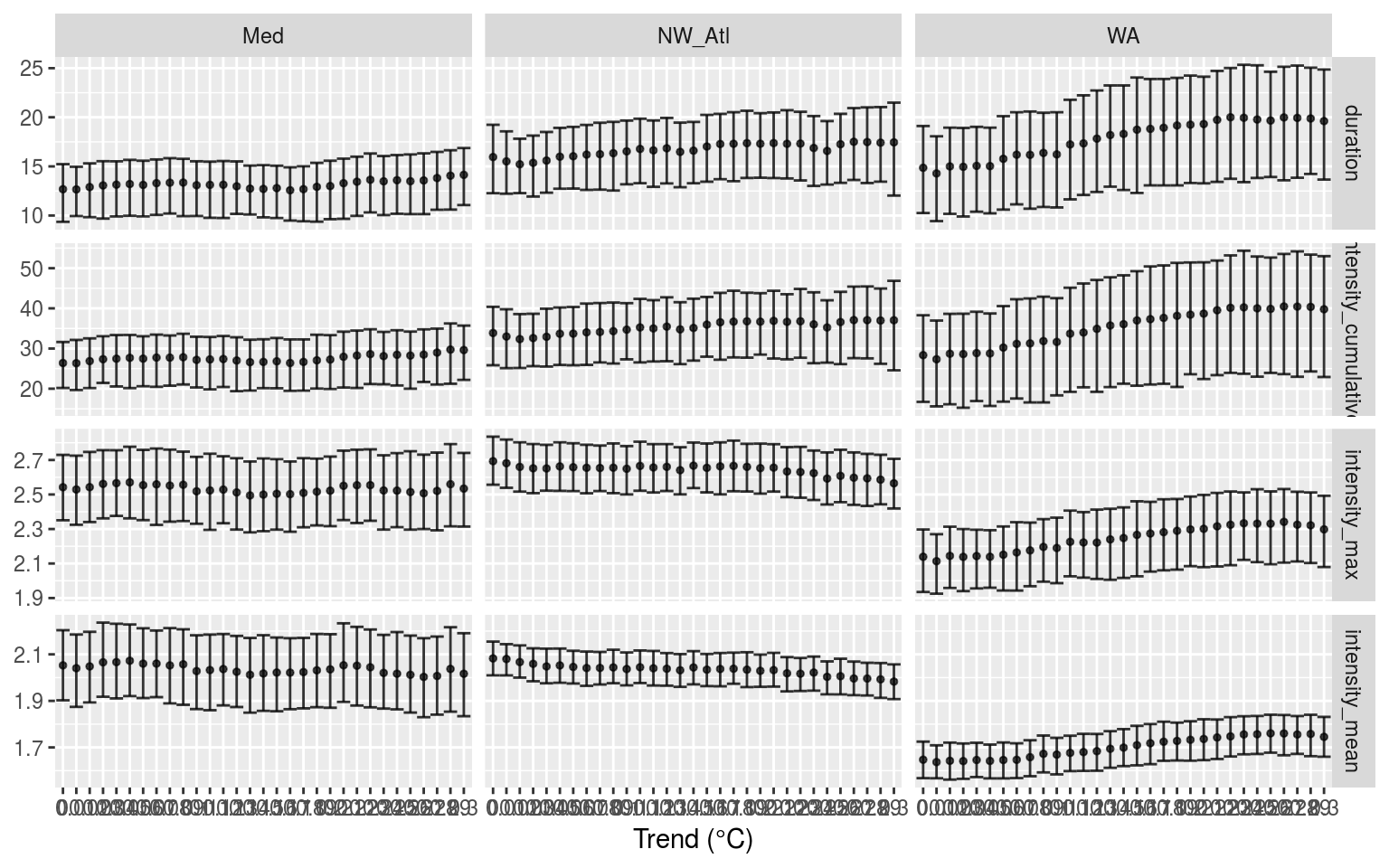
Confidence intervals of the MHW metrics when increasing decadal trends were added.
# CI_plot_1Because this set of data is smaller than the previous two vignettes I have used basic bootstrapping to create the CIs above. From these we see that the duration and int. cum. of all of the time series tend to increase as the decadal trend increase, but this is never significant. The patterns for mean and max int. are different for each time series. The Med remains relatively flat regardless of decadal trend, WA increases, and NW_Atl decreases. This is likely due to the distribution of MHWs throughout the time series.
Categories
chi-squared
In order to detemine if the count of MHWs, both total and individual categories, differs based on the decadal trends present in the data, we will be performing a series of chi-squared tests for each site.
# Simple wrapper for nesting
# df <- sst_ALL_trend_cat_all %>%
#   filter(site == "WA")
chi_p <- function(df){
  res <- chisq.test(table(df$trend, df$category), correct = FALSE)
  res_tidy <- broom::tidy(res)
  return(res_tidy$p.value)
}

# Load and extract category data
load("data/sst_ALL_trend_clim_event_cat.Rdata")
suppressWarnings( # Suppress warning about category levels not all being present
sst_ALL_trend_cat <- sst_ALL_trend_clim_event_cat %>%
  select(-events) %>%
  unnest()
)

# Get data into the expected format
sst_ALL_trend_cat_total <- sst_ALL_trend_cat %>%
  select(trend, site, category) %>%
  mutate(category = "total")

sst_ALL_trend_cat_all <- sst_ALL_trend_cat %>%
  select(trend, site, category) %>%
  rbind(sst_ALL_trend_cat_total)

# Calculate chi-squared p-value
sst_ALL_trend_cat_chi <- sst_ALL_trend_cat_all %>%
  group_by(site) %>%
  nest() %>%
  mutate(p.value = map(data, chi_p)) %>%
  select(-data) %>%
  unnest()

save(sst_ALL_trend_cat_chi, file = "data/sst_ALL_trend_cat_chi.Rdata")
load("~/MHWdetection/analysis/data/sst_ALL_trend_cat_chi.Rdata")
knitr::kable(sst_ALL_trend_cat_chi, caption = "Table showing the significant difference (_p_-value) for the count of different categories of events for each site based on the trends introduced into the data. No differences were found.")| site | p.value |
|---|---|
| Med | 1 |
| NW_Atl | 1 |
| WA | 1 |
Session information
sessionInfo()R version 3.5.3 (2019-03-11)
Platform: x86_64-pc-linux-gnu (64-bit)
Running under: Ubuntu 16.04.5 LTS
Matrix products: default
BLAS: /usr/lib/openblas-base/libblas.so.3
LAPACK: /usr/lib/libopenblasp-r0.2.18.so
locale:
[1] LC_CTYPE=en_CA.UTF-8 LC_NUMERIC=C
[3] LC_TIME=en_CA.UTF-8 LC_COLLATE=en_CA.UTF-8
[5] LC_MONETARY=en_CA.UTF-8 LC_MESSAGES=en_CA.UTF-8
[7] LC_PAPER=en_CA.UTF-8 LC_NAME=C
[9] LC_ADDRESS=C LC_TELEPHONE=C
[11] LC_MEASUREMENT=en_CA.UTF-8 LC_IDENTIFICATION=C
attached base packages:
[1] stats graphics grDevices utils datasets methods base
other attached packages:
[1] bindrcpp_0.2.2 ggridges_0.5.0 mgcv_1.8-24
[4] nlme_3.1-137 FNN_1.1.2.1 boot_1.3-20
[7] ggpubr_0.1.8 magrittr_1.5 fasttime_1.0-2
[10] lubridate_1.7.4 heatwaveR_0.3.6.9003 data.table_1.11.6
[13] broom_0.5.0 forcats_0.3.0 stringr_1.3.1
[16] dplyr_0.7.6 purrr_0.2.5 readr_1.1.1
[19] tidyr_0.8.1 tibble_1.4.2 ggplot2_3.0.0
[22] tidyverse_1.2.1
loaded via a namespace (and not attached):
[1] tidyselect_0.2.4 reshape2_1.4.3 haven_1.1.2
[4] lattice_0.20-35 colorspace_1.3-2 viridisLite_0.3.0
[7] htmltools_0.3.6 yaml_2.2.0 plotly_4.8.0
[10] rlang_0.2.2 R.oo_1.22.0 pillar_1.3.0
[13] glue_1.3.0 withr_2.1.2 R.utils_2.7.0
[16] modelr_0.1.2 readxl_1.1.0 bindr_0.1.1
[19] plyr_1.8.4 munsell_0.5.0 gtable_0.2.0
[22] workflowr_1.1.1 cellranger_1.1.0 rvest_0.3.2
[25] R.methodsS3_1.7.1 htmlwidgets_1.2 evaluate_0.11
[28] labeling_0.3 knitr_1.20 highr_0.7
[31] Rcpp_0.12.18 scales_1.0.0 backports_1.1.2
[34] jsonlite_1.5 hms_0.4.2 digest_0.6.16
[37] stringi_1.2.4 grid_3.5.3 rprojroot_1.3-2
[40] cli_1.0.0 tools_3.5.3 lazyeval_0.2.1
[43] crayon_1.3.4 whisker_0.3-2 pkgconfig_2.0.2
[46] Matrix_1.2-14 xml2_1.2.0 assertthat_0.2.0
[49] rmarkdown_1.10 httr_1.3.1 rstudioapi_0.7
[52] R6_2.2.2 git2r_0.23.0 compiler_3.5.3 This reproducible R Markdown analysis was created with workflowr 1.1.1