%load_ext load_style
%load_style talk.css
Numpy
import addutils.toc ; addutils.toc.js(ipy_notebook=True)
from IPython.display import Image, HTML
Numpy is the fundamental building block of the so-called Python Scientific Stack
It provides a special data structure, the numpy ndarray (N - dimensional array) which allows the representation of arrays of numerical values, integers, reals, complex
Numpy arrays by default can only hold objects of the same type (e.g. cannot mix integers and floats))
It also provides with random number capability, some convenience simple statistical functions (mean, std, ...) and some essential linear algebra operations
HTML("<iframe src='http://numpy.org/' width=1000 height=500></iframe>")
The conventional way to import numpy is
import numpy as np
import numpy as np
import matplotlib.pyplot as plt
%matplotlib inline
Numpy basics
Constructing an numpy array
x = [1,2,3,4] # x is a regular python list
type(x)
x = np.array(x)
type(x)
a = np.array(range(10))
a
x = [[1,2,3],[4,5,6]] # nested lists
x = np.array(x)
x
x.shape
The shape attribute is a tuple containing the dimensions along each axis (0 = rows, 1 = columns, ...)
x = np.arange(1000).reshape((10,10,10))
x.shape
Be careful: keep in mind references Vs. copies of arrays!
a
x = a
x
a[2] = 99
a
x
x has changed !, because x = a only means you create a new reference pointing to the same object as the array a
We can see that by using the id function, which returns the object's memory adress
id(a)
id(x)
If you want to create a copy instead of a reference, you need to do it explicitely
x = a.copy()
id(x)
a[3] = 888
a
x
Numpy array types
Numpy tries and guess the correct type of the numerical values if you pass a list, here x is of type integer 64
x.dtype
You can change that using the method astype()
x = x.astype(np.float)
x.dtype
x
you can mix different types when creating an array from a list, but numpy will cast all values to the safest dtype
x = np.array([1.0,1,1])
x
You can (but why would you ?) create arrays of native Python types, i.e. here an array containing a dictionnary and a tuple
x = np.array([{'A':1},(1,3)])
In that case the dtype is Object ('O')
x
Some convenience functions for creating arrays
np.arange(start, stop, step, dtype=None)
np.arange(100).shape
np.arange(0,100+10,10)
np.linspace(start, stop, num=50, *endpoint=True*, *retstep=False*)
np.linspace(0,0.5,10, endpoint=False)
same as np.arange(0,0.5, 0.05)
np.arange(0,0.5,0.05)
np.ones(shape, dtype=None, order='C') creates an array of ones, similar function is np.zeros
np.ones((10,12))
np.empty can be used to pre-allocate "empty" arrays with small memory footprint
np.empty((5,5))
Array indexing
Simple indexing
a = np.arange(25,dtype=float).reshape(5,5) # creating a 2D array, note the dtype
print(a)
a.shape
a[0,1] # FIRST row, SECOND column, remember, Python indexing is zero-based
a[:,0] # first column
a[1,:] # second row
a[:,2:] # all rows from third colum
a[-1,:] # last row
a[:,::-1] # handy: reverses column order
a
slices allows to easily select contiguous row / colums
a[0:2,1:3] # first two rows, and columns 2 to 3
When you want to select non-contiguous (or repeated) rows / columns, you can use the ix_ construct
a[np.ix_([0,1,3],[1,1,3])]
a
Boolean or conditional indexing
a = a[a>10]
print(a)
Array broadcasting
Simple possible case: scalar broadcasting
x = np.array([0,1,2,3]); print(x)
x.shape
x + 3
2D broadcasting
x = np.arange(12).reshape((3,4))
x
x.shape
y = np.arange(3).reshape((3,1)); # or y = np.arange(3)[np.newaxis,:] or y = np.arange(3)[None,:]
y.shape
x + y
3D broadcasting
x = np.arange(15).reshape((3, 5))
x.shape
y = np.ones(8)
z = x[...,np.newaxis] + y
print(z)
z.shape
Array methods
We have already seen some array methods above, in this section I just dwelve into their general behavior and present some convenient array methods
In python, everything is an object, numpy ndarrays are no exceptions, and they expose a number of methods, which are equivalent to the call the respective numpy function, but can be more convenient to use, and - marginally - faster
a.shape # shape of a (like *size* in matlab)
np.shape(a)
%timeit a.mean() # The %timeit magic cell function times the execution of an expression
%timeit np.mean(a)
b = np.arange(100,dtype=float).reshape(10,10) # creating a 2D array, note the dtype
b.shape
b
b.sum(0) ### summing over the first axis ('rows')
np.sum(b, axis=0)
b[:,0].sum()
swapaxes method swap the position of 2 axes
b = b.swapaxes(1,0)
b
here equivalent to transpose() on 2D array
b = b.transpose()
b
b = np.transpose(b)
b
argsort, argmin and argmax returns the indices that would sort an array (along an axis), and the indices of min and max values
a = np.array([11,13,15,17,19,18,16,14,12,10])
a.argsort()
a.sort(); print(a)
array functions
we've seen above array methods, available through the object-oriented interface of Python, now we're gonna see a few useful numpy functions
from scipy import misc
img = misc.ascent()
img.shape
plt.imshow(img, cmap=plt.get_cmap('gray'))

plt.imshow(np.tile(img, (2,1)), cmap=plt.get_cmap('gray'))

plt.imshow(np.tile(img, (1,2)), cmap=plt.get_cmap('gray'))

plt.imshow(np.repeat(img, 2, axis=1), cmap=plt.get_cmap('gray'))

plt.imshow(np.resize(img, (750,512)), cmap=plt.get_cmap('gray'))

Universal functions
A universal function (or ufunc for short) is a function that operates on ndarrays in an element-by-element fashion, supporting array broadcasting, type casting, and several other standard features. That is, a ufunc is a “vectorized” wrapper for a function that takes a fixed number of scalar inputs and produces a fixed number of scalar outputs.
x = np.sin(np.linspace(-2*np.pi, 2*np.pi, 10000).reshape((100,100)))
plt.imshow(x, cmap=plt.get_cmap('gray_r'))

vectorization
def max100(x):
    """
    returns the max between x and 100
    """

    return(max(x,100))
x = np.random.normal(loc=50, scale=100, size=(10,10))
x
max100(x)
that fails because max100 is just a regular python function, that expects a single object
but we can build easily a vectorized version of the same function (i.e. building a ufuncmm)
vmax100 = np.vectorize(max100)
z = vmax100(x)
z.shape
z
Numpy provides a number of already vectorized mathematical functions (ufuncs again). e.g. round, fix and all basic trigonometric (sin, cos, tan, sic), exponential (exp, exp2, sinh, cosh), and logarithmic functions (log, log10, log2).
Missing values in numpy
You can handle missing values in Numpy in two different ways:
- By using the np.nan (not a number) special type
- By casting a numpy array into a Masked array using the ma module
Using the masked array approach, while somehow more cumbersome, allows more flexibility
from numpy import ma
b[5,5] = -999.
print(b)
c = b.copy()
c[c == -999.] = np.nan
print(c)
nan values propagates automatically when using aggregation functions
c.mean(1)
Unless you use one of the - few - NaN functions
np.nansum(c,axis=1)
Now we're gonna see how to use the ma (Masked Arrays) module
b = ma.masked_values(b, -999.)
print(b)
b has now two new attributes: data, and mask
print(b.data)
print(b.mask)
b.mean(1)
c = b.mean(1)
c.shape
Masked values are just ignored in calculations
Other masked array functions allow to set masked values according to some conditions, all (I think) functions exposed for regular numpy arrays are available.
b = ma.
b
b.mean(0)
Random numbers
You can generate random numbers coming from a wide range of distributions
np.random.
If you want more distributions, and more flexibility, you need to look into scipy.stats.distributions (see the statistical modelling notebook)
Example 1: Normal distribution
$$P(x) = \frac{1}{\sqrt{2\pi\sigma^2}}\exp\left[-\frac{(x-\mu)^2}{2\sigma^2}\right]$$x = np.random.normal(0,1,1000)
x = np.random.standard_normal(1000)
_ = plt.hist(x, color='0.6',normed=True)

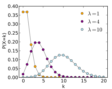
Example 2: Poisson distribution
\begin{equation*} P\left( x \right) = \frac{{e^{ - \lambda } \lambda ^x }}{{x!}} \end{equation*}poiss = np.random.poisson(lam=4, size=(10000))
#a = np.array([len(np.where(poiss==x)[0]) for x in np.unique(poiss)])
a = np.array([sum(poiss==x) for x in np.unique(poiss)])
f, ax = plt.subplots()
ax.plot(np.unique(poiss), a/10000., '-', color='grey')
ax.plot(np.unique(poiss), a/10000., 'o', color='purple', markersize=10)
ax.set_title("Poisson Empirical PMF, $\lambda = 4$", fontsize=20)
ax.set_xlim(-1,17)
ax.set_ylim(0,0.25)
[l.set_fontsize(16) for l in ax.xaxis.get_ticklabels()]
[l.set_fontsize(16) for l in ax.yaxis.get_ticklabels()];

import math # the math module exposes mathematical functions operating on scalars
lam = 4; end = 20 # lambda is a reserved word in python
P = [math.exp(-lam)*lam**x/math.factorial(x) for x in range(end)] # note the use of a list comprehension
f, ax = plt.subplots()
ax.plot(P, '-', color='grey')
ax.plot(P, 'o', color='purple', markersize=10)
ax.set_title("Poisson PMF, $\lambda = 4$", fontsize=20)
ax.set_xlim(-1,17)
ax.set_ylim(0,0.25)
[l.set_fontsize(16) for l in ax.xaxis.get_ticklabels()]
[l.set_fontsize(16) for l in ax.yaxis.get_ticklabels()];

From Wikipedia (http://en.wikipedia.org/wiki/Poisson_distribution)