Promoter Architecture
Philipp Ross
09-25-2018
Last updated: 2018-09-30
Code version: 3e6a944
Sequence features surrounding transcription start sites
For this analysis we want to plot nucleotide frequencies up and downstream of predicted TSSs. We can do this by looking at most commonly used TSSs, tag clusters, and promoter clusters.
First we’ll import all the data:
# import genome
library(BSgenome.Pfalciparum.PlasmoDB.v24)

# import tag clusters
tc_intergenic <- rtracklayer::import.gff3("../output/ctss_clustering/modified/tag_clusters_annotated_intergenic.gff")
tc_exonic     <- rtracklayer::import.gff3("../output/ctss_clustering/modified/tag_clusters_annotated_exons.gff")
tc_intronic   <- rtracklayer::import.gff3("../output/ctss_clustering/modified/tag_clusters_annotated_introns.gff")

# import promoter clusters
pc_intergenic <- rtracklayer::import.gff3("../output/ctss_clustering/modified/promoter_clusters_annotated_intergenic.gff")
pc_exonic     <- rtracklayer::import.gff3("../output/ctss_clustering/modified/promoter_clusters_annotated_exons.gff")
pc_intronic   <- rtracklayer::import.gff3("../output/ctss_clustering/modified/promoter_clusters_annotated_introns.gff")

# import telomere ranges
telomeres  <- rtracklayer::import.gff3("../data/annotations/Pf3D7_v3_subtelomeres.gff")

# import genes as well
genes <- rtracklayer::import.gff3("../data/annotations/genes_nuclear_3D7_v24.gff")

distance_to_add <- 500

# original TSO-predicted TSSs
x3d7_tso <- rtracklayer::import.gff3("../data/utrs/original_utrs/tso_thr5.gff") %>%
  tibble::as_tibble() %>%
  dplyr::mutate(newend=ifelse(strand=="+",start+distance_to_add,end+distance_to_add),
                newstart=ifelse(strand=="+",start-distance_to_add,end-distance_to_add)) %>%
  dplyr::select(-start,-end) %>%
  dplyr::rename(start=newstart,end=newend) %>%
  dplyr::filter(type=="5UTR") %>%
  GenomicRanges::GRanges()

# import most heavily used TSSs
x3d7_tss <- rtracklayer::import.gff3("../output/final_utrs/final_utrs_3d7.gff") %>%
  tibble::as_tibble() %>%
  dplyr::mutate(newend=ifelse(strand=="+",start+distance_to_add,end+distance_to_add),
                newstart=ifelse(strand=="+",start-distance_to_add,end-distance_to_add)) %>%
  dplyr::select(-start,-end) %>%
  dplyr::rename(start=newstart,end=newend) %>%
  dplyr::filter(type=="5UTR") %>%
  GenomicRanges::GRanges()

# import TTS for 3D7
x3d7_tts <- rtracklayer::import.gff3("../output/final_utrs/final_utrs_3d7.gff") %>%
  tibble::as_tibble() %>%
  dplyr::mutate(newend=ifelse(strand=="+",end+distance_to_add,start+distance_to_add),
                newstart=ifelse(strand=="+",end-distance_to_add,start-distance_to_add)) %>%
  dplyr::select(-start,-end) %>%
  dplyr::rename(start=newstart,end=newend) %>%
  dplyr::filter(type=="3UTR") %>%
  GenomicRanges::GRanges()

# HB3
xhb3_tss <- rtracklayer::import.gff3("../output/final_utrs/final_utrs_hb3.gff") %>%
  tibble::as_tibble() %>%
  dplyr::mutate(newend=ifelse(strand=="+",start+distance_to_add,end+distance_to_add),
                newstart=ifelse(strand=="+",start-distance_to_add,end-distance_to_add)) %>%
  dplyr::select(-start,-end) %>%
  dplyr::rename(start=newstart,end=newend) %>%
  dplyr::filter(type=="5UTR") %>%
  GenomicRanges::GRanges()

# IT
xit_tss <- rtracklayer::import.gff3("../output/final_utrs/final_utrs_it.gff") %>%
  tibble::as_tibble() %>%
  dplyr::mutate(newend=ifelse(strand=="+",start+distance_to_add,end+distance_to_add),
                newstart=ifelse(strand=="+",start-distance_to_add,end-distance_to_add)) %>%
  dplyr::select(-start,-end) %>%
  dplyr::rename(start=newstart,end=newend) %>%
  dplyr::filter(type=="5UTR") %>%
  GenomicRanges::GRanges()
Let’s set the nucleotide colors to be what we want them to be:
# set colors
set_colors <- function(colors, vars, iname) {
  myColors <- c(colors)
  names(myColors) <- levels(vars)
  output <- ggplot2::scale_colour_manual(name = iname, values = myColors)
  return(output)
}
# custom nucleotide colors
base_colors <- set_colors(c("#E41A1C", "#377EB8", "#F0E442", "#4DAF4A"),
                          c("A", "T", "C", "G"), "base")
Now let’s write the functions to generate the frequency diagrams, information content, and sequence logos:
# Use this function to generate position weight matrices
generate_pwm <- function(clusters) {
# extract sequences from the genome
seqs <- BSgenome::getSeq(BSgenome.Pfalciparum.PlasmoDB.v24,clusters)
# convert those sequences into a data frame
tmp <- lapply(seqs,function(x) stringr::str_split(as.character(x),"")[[1]])
tmp <- as.data.frame(tmp)
colnames(tmp) <- 1:ncol(tmp)
tmp$pos <- 1:nrow(tmp)
tmp <- tmp %>% tidyr::gather(seq, base, -pos)
# calculate the proportion of nucleotides at each position
pwm <- tmp %>%
dplyr::group_by(as.numeric(pos)) %>%
dplyr::summarise(A = sum(base == "A")/n(),
C = sum(base == "C")/n(),
G = sum(base == "G")/n(),
T = sum(base == "T")/n()) %>%
dplyr::ungroup()
colnames(pwm)[1] <- "pos"
return(list(pwm=pwm,seqs=seqs))
}
# Plot the nucleotide frequencies at each position
plot_frequencies <- function(ipwm) {
ipwm %>%
tidyr::gather(base, freq, -pos) %>%
ggplot(aes(x = pos, y = freq, color = base)) +
geom_line(size = 1) +
geom_point(size = 1.5) +
xlab("") +
ylab("Frequency") +
scale_y_continuous(limits = c(0,1)) +
theme(legend.position="top",
legend.direction="horizontal",
legend.title = element_blank()) +
base_colors
}
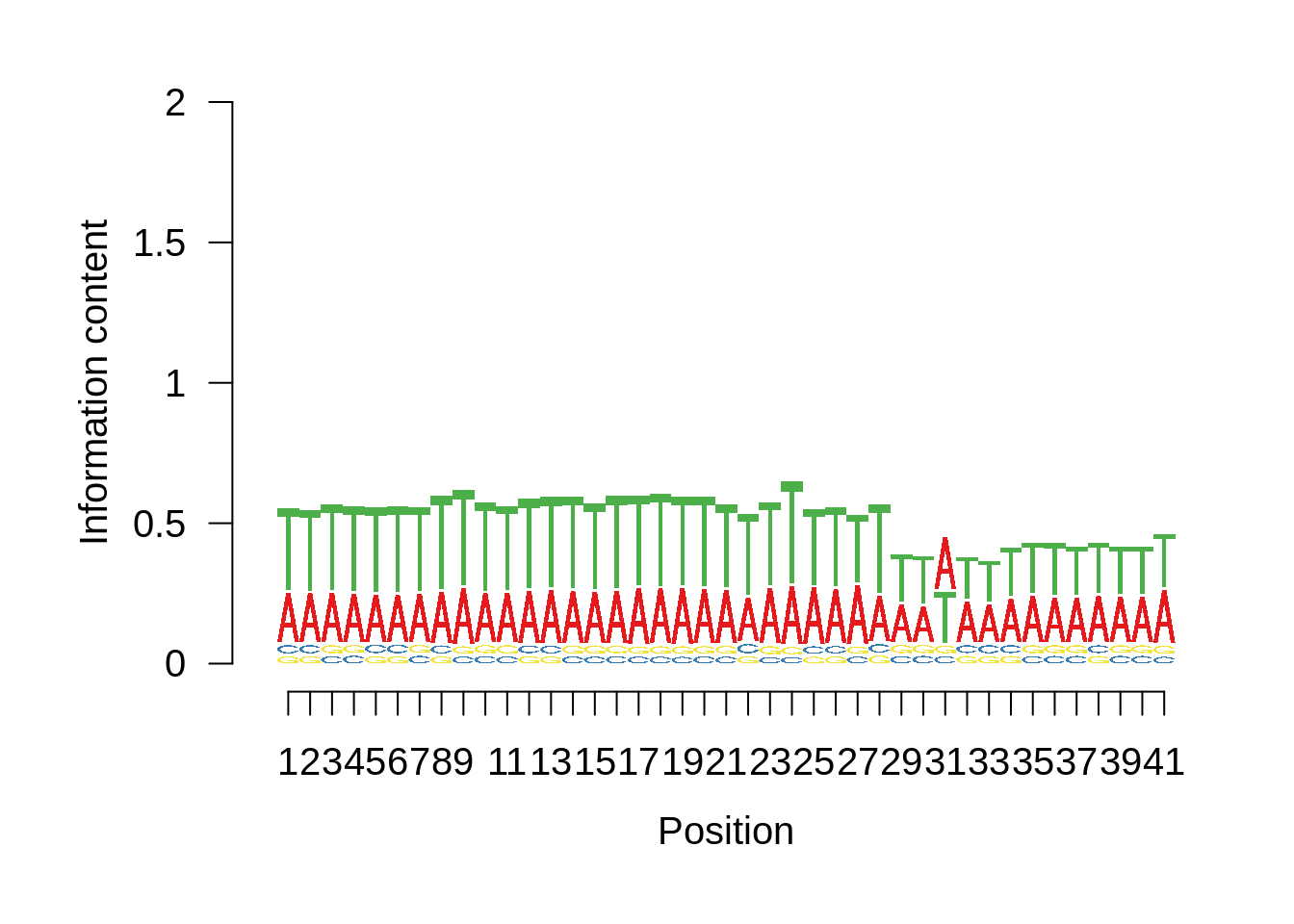
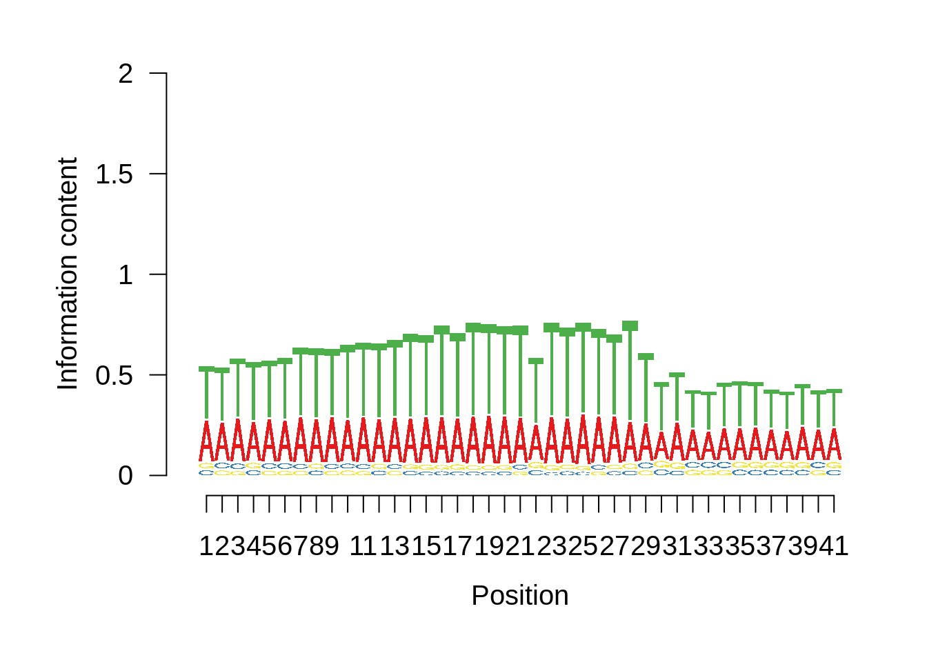
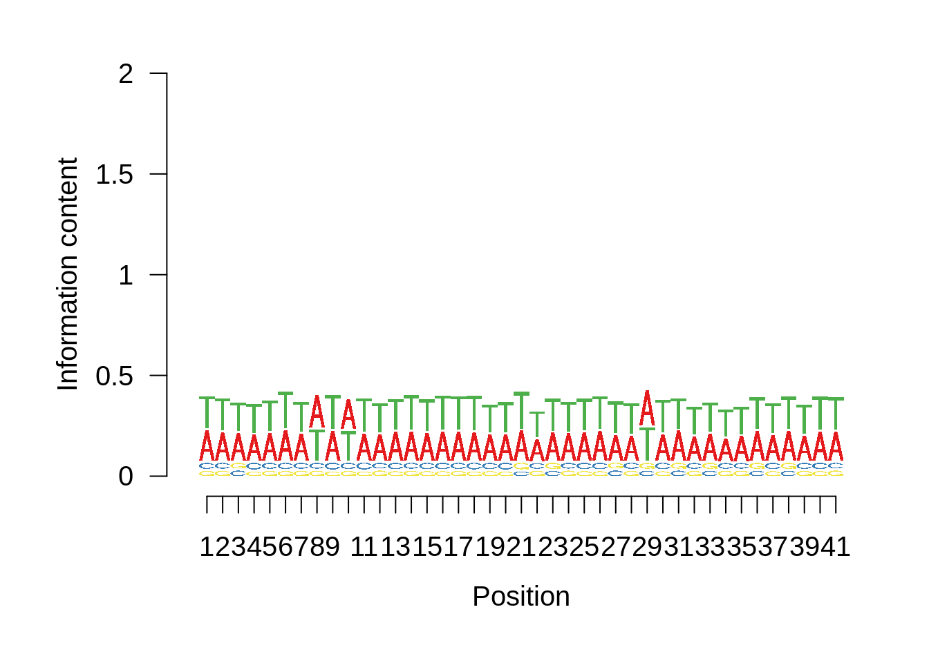
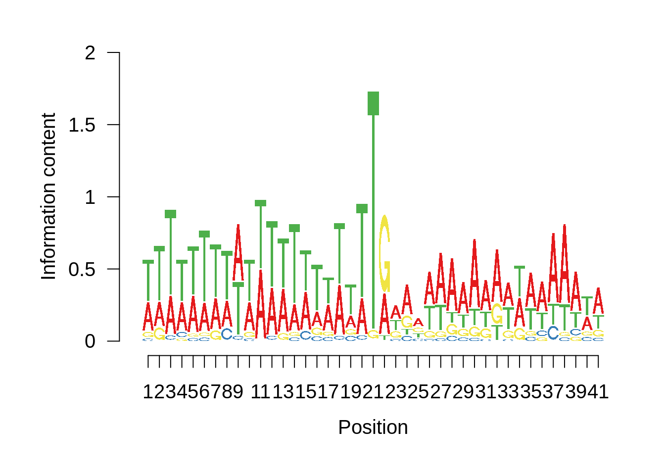
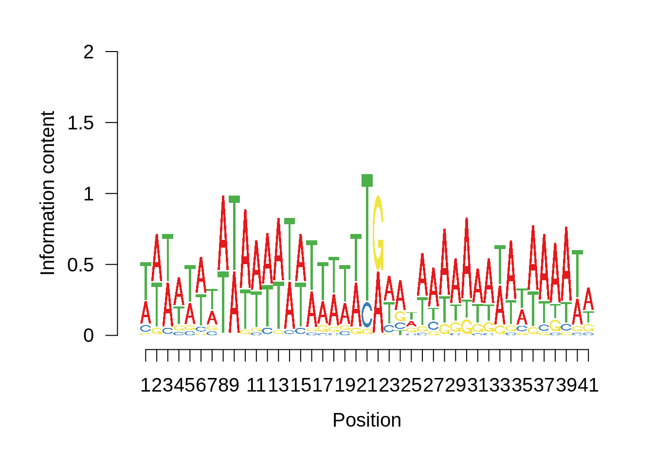
# Plot the sequence logo
plot_logo <- function(ipwm,limits) {
logo <- ipwm[,2:5]
seqLogo::seqLogo(seqLogo::makePWM((t(logo[limits[1]:limits[2],]))),ic.scale = T)
}
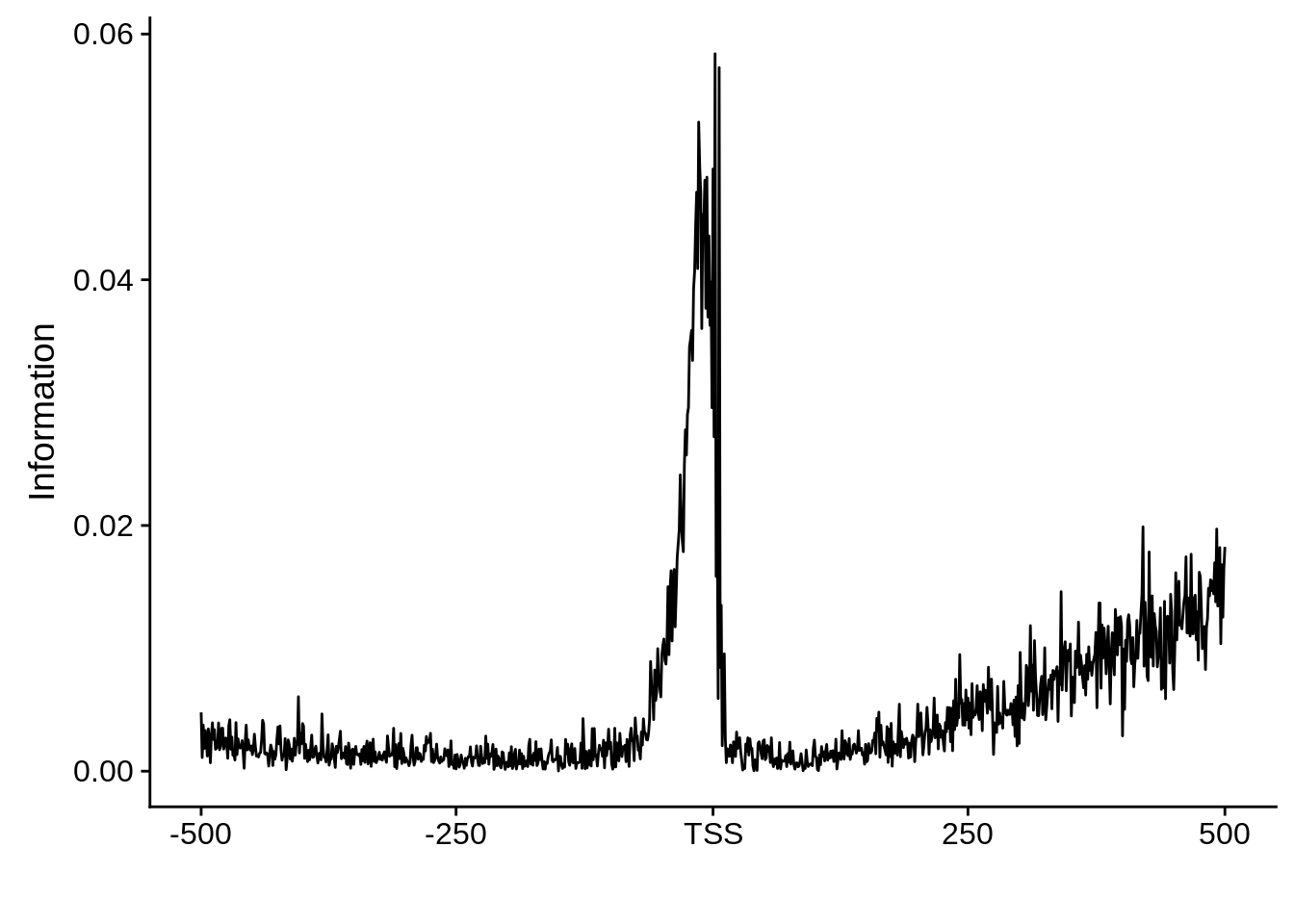
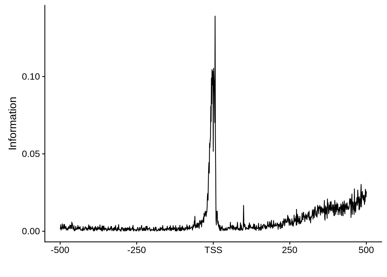
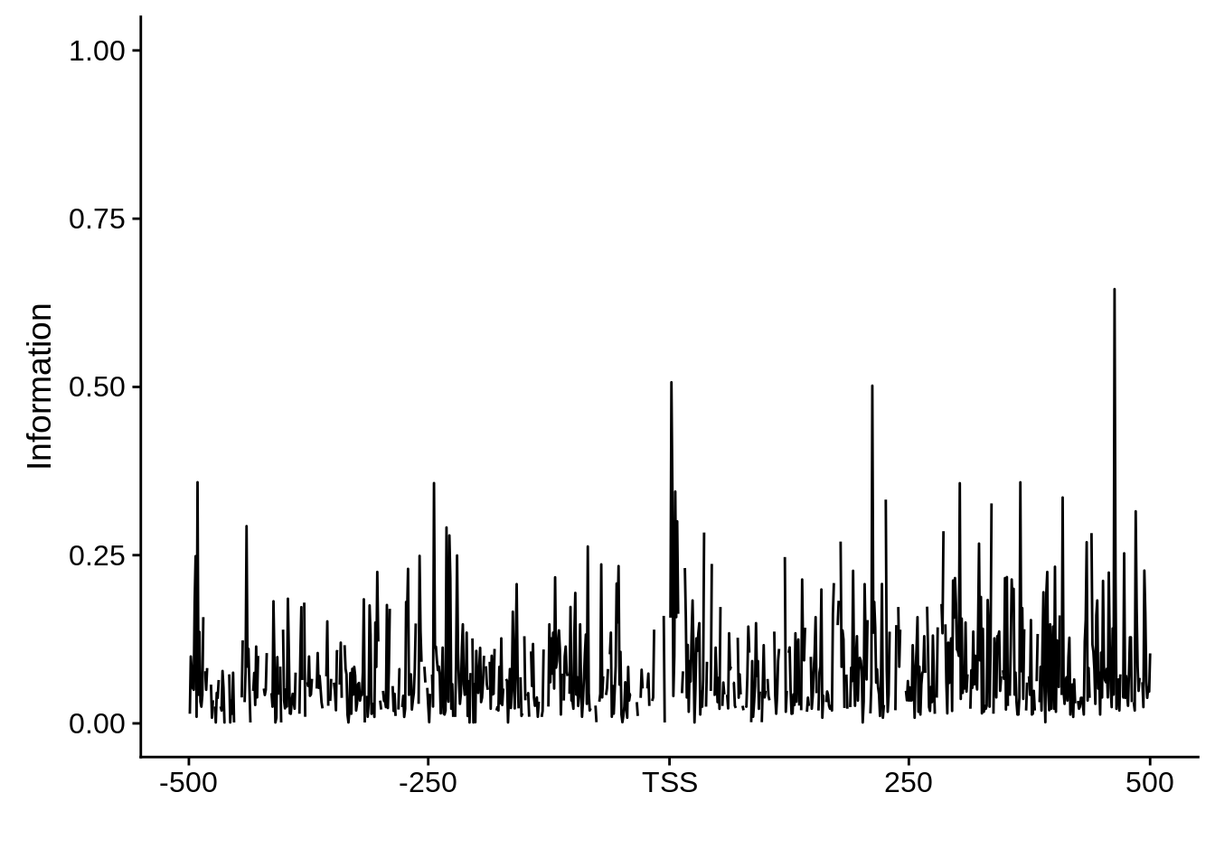
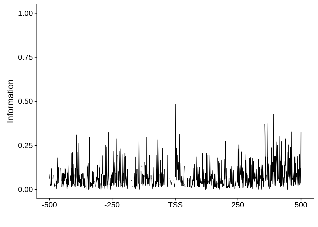
# Plot the information content at each position
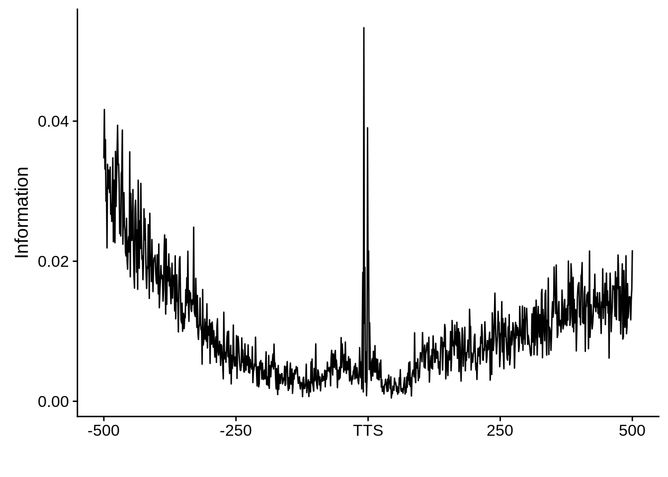
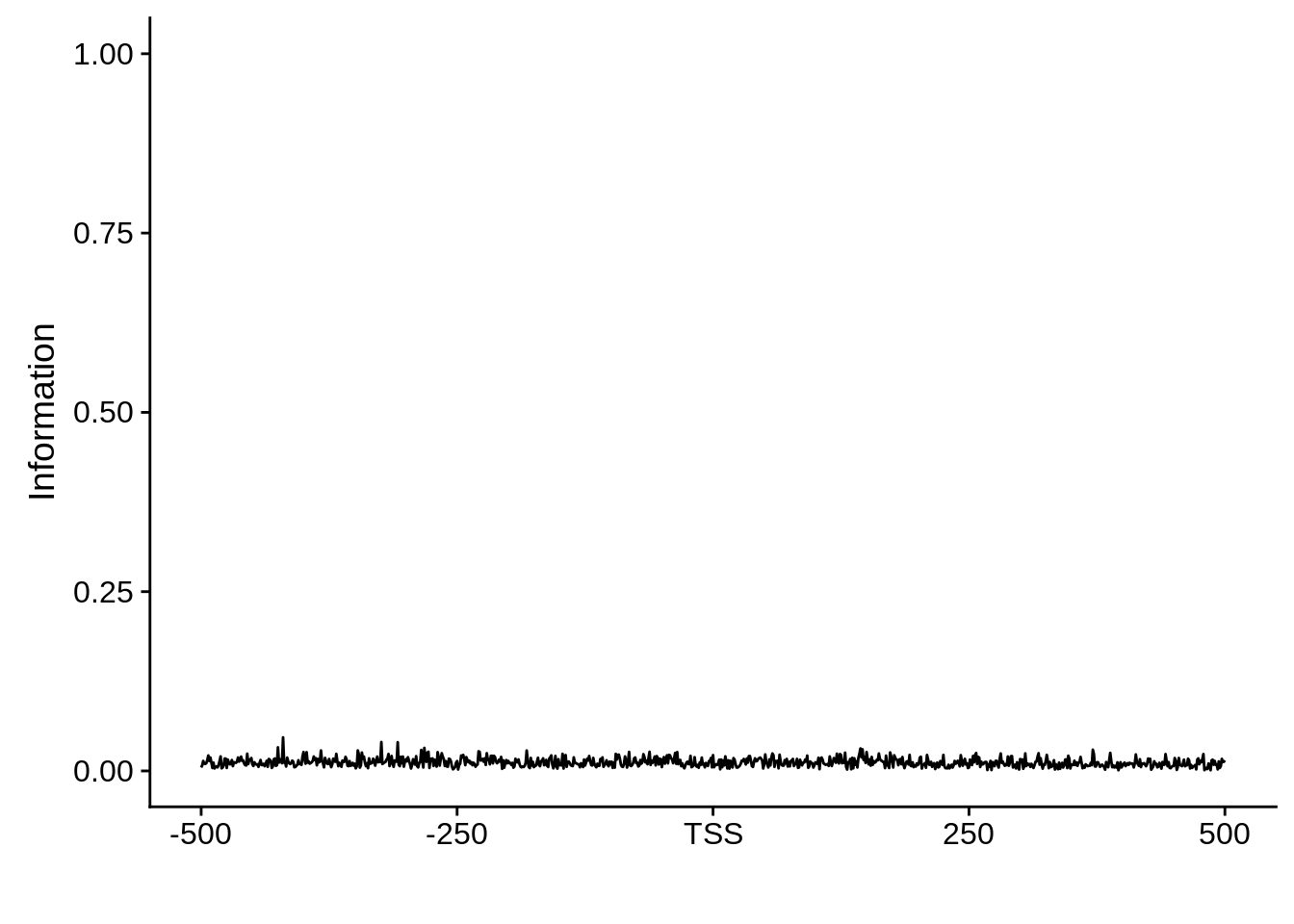
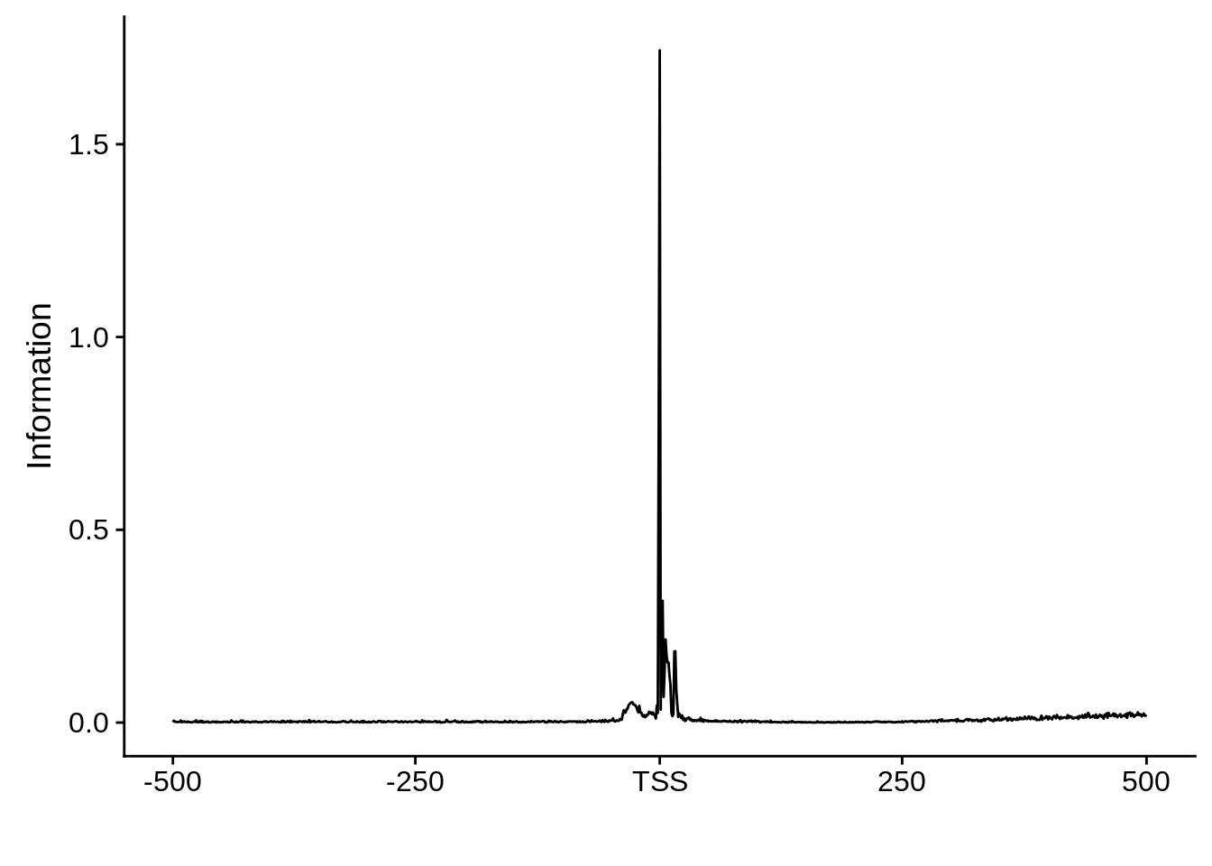
plot_info <- function(ipwm) {
ipwm %>%
dplyr::mutate(i = (A * log2(A/0.42)) + (T * log2(T/0.45)) + (G * log2(G/0.07)) + (C * log2(C/0.06))) %>%
gather(base, freq, -pos, -i) %>%
ggplot(aes(x = pos, y = i)) +
geom_line() +
xlab("") +
ylab("Information")
}And now we can start making some plots.
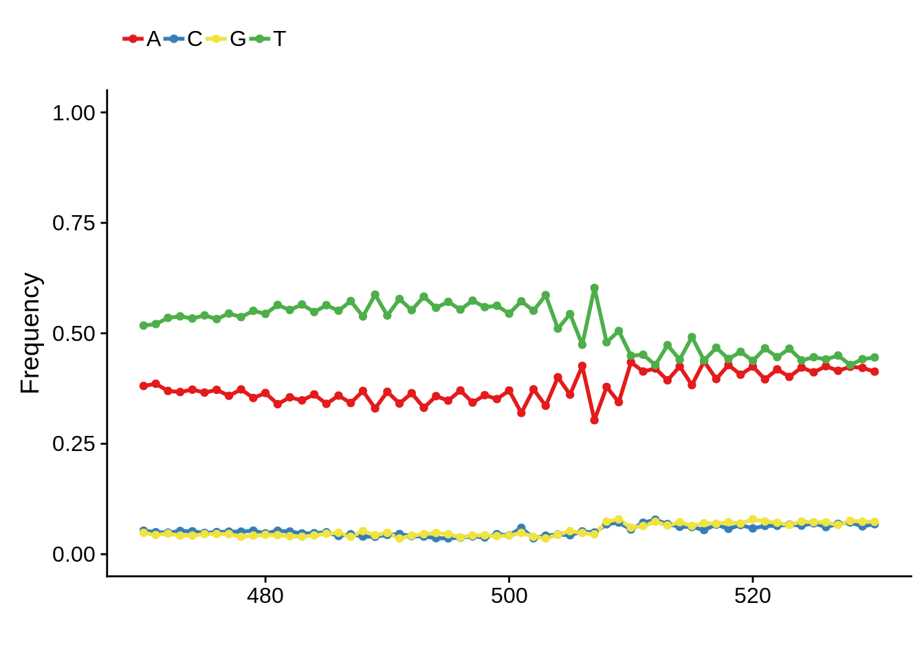
Most commonly used 5’ TSS
First, we can look at the most commonly used TSSs for each strain:
3D7
x3d7pwm <- generate_pwm(x3d7_tss)
plot_frequencies(x3d7pwm$pwm) + scale_x_continuous(limits=c(480,520))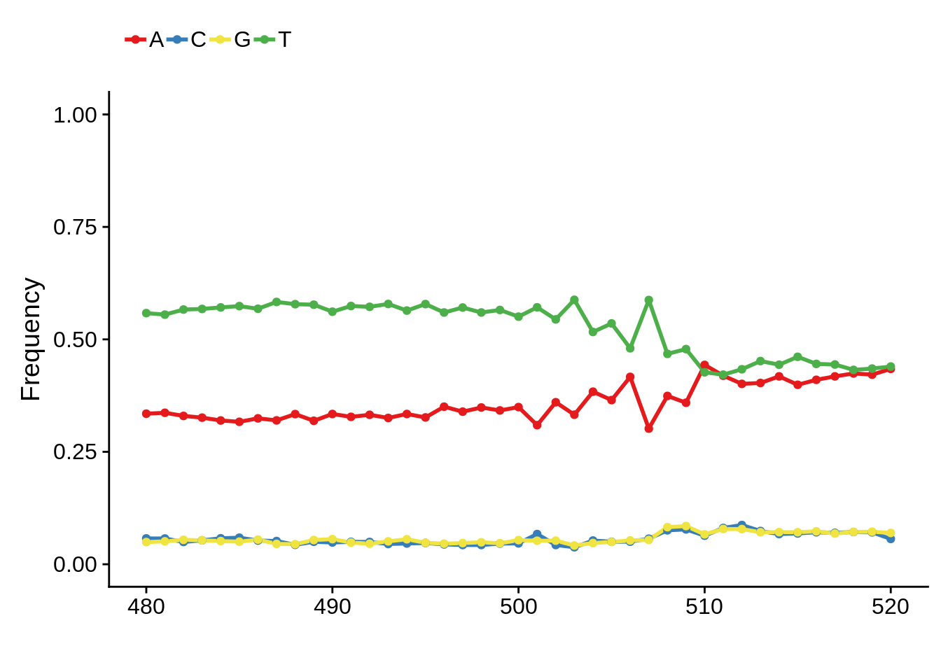
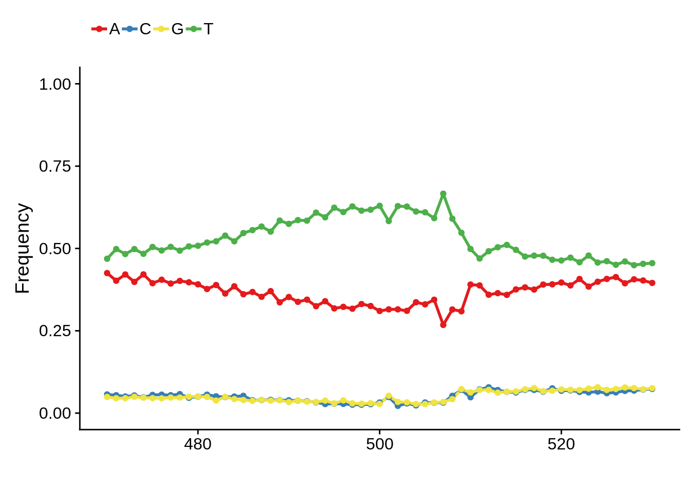
Most commonly used 3’ TTS
We can also look at the most commonly used TTS in 3D7:
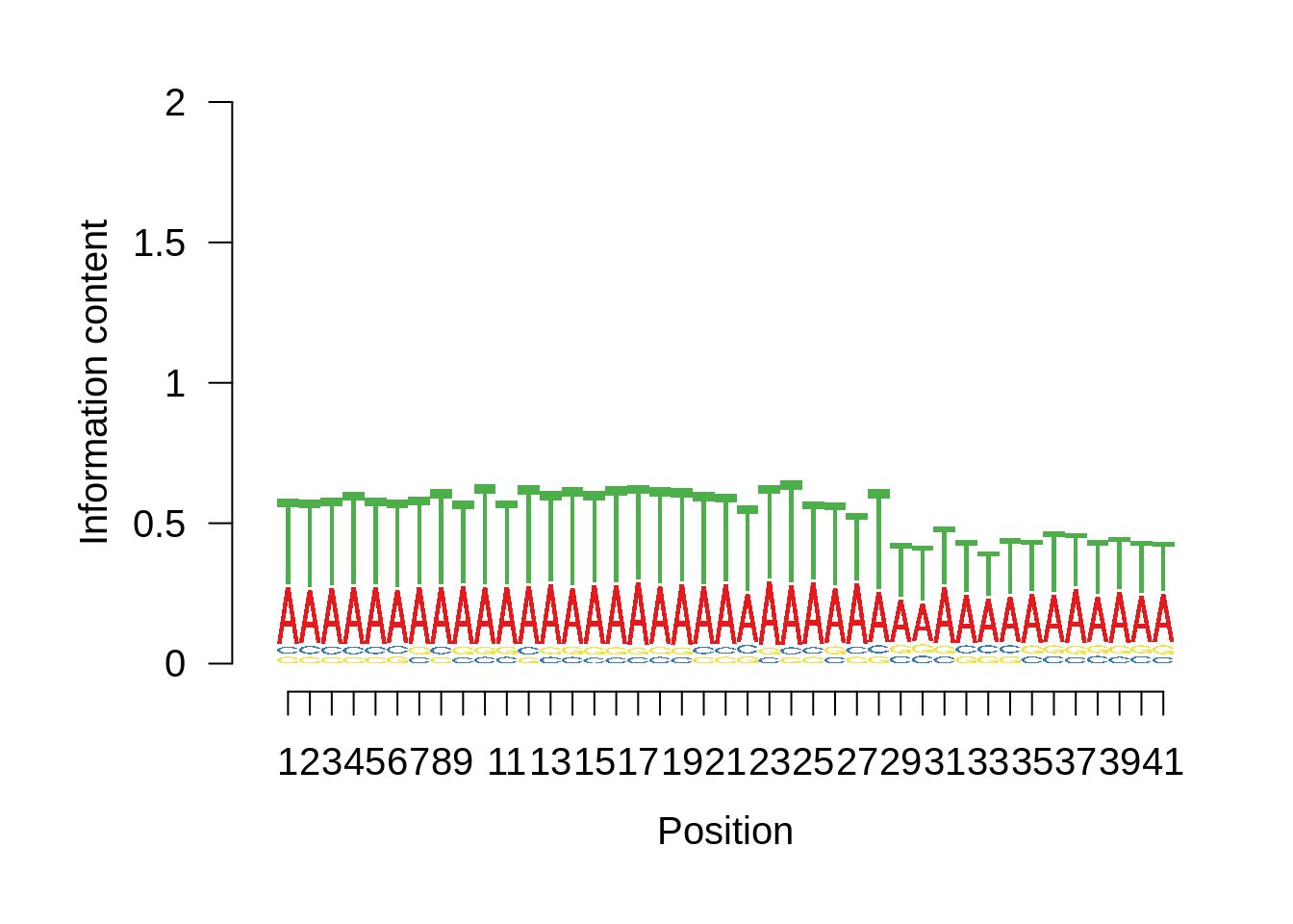
x3d7pwm <- generate_pwm(x3d7_tts)
plot_frequencies(x3d7pwm$pwm) + scale_x_continuous(limits=c(470,530))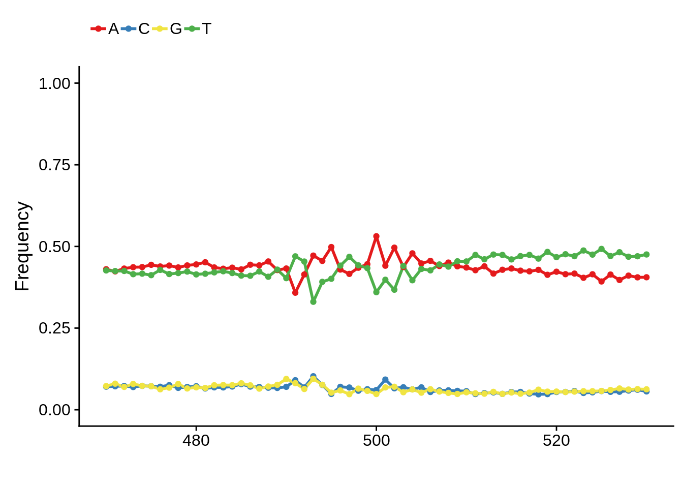
We can also compare this to random intergenic sequences:
set.seed(33)
intergenic <- GenomicRanges::gaps(genes)
intergenic <- intergenic[is.na(GenomicRanges::findOverlaps(intergenic,telomeres,select="arbitrary"))]
intergenic_seqs <- BSgenome::getSeq(BSgenome.Pfalciparum.PlasmoDB.v24,intergenic)

# create random seqs to compare to
extract_random_seqs1 <- function(seqs,widths) {
  # start with the first sequence,
  # filter by width to avoid errors,
  # sample randomly from filtered sequences,
  # grab random interval that matches the length of the
  # promoter sequence
  fseqs       <- seqs[width(seqs) > widths[1]]
  rsample     <- sample(1:length(fseqs),size=1)
  rseq        <- fseqs[rsample][[1]]
  rstart      <- sample(x=1:(length(rseq)-widths[1]),size=1)
  random_seqs <- rseq[rstart:(rstart+widths[1]-1)]
  # do this for all sequences
  for (i in 2:length(widths)) {
    fseqs       <- seqs[width(seqs) > widths[i]]
    rsample     <- sample(1:length(fseqs),size=1)
    rseq        <- fseqs[rsample][[1]]
    rstart      <- sample(x=1:(length(rseq)-widths[i]-1),size=1)
    random_seqs <- unlist(Biostrings::DNAStringSetList(
      Biostrings::DNAStringSet(random_seqs),
      Biostrings::DNAStringSet(rseq[rstart:(rstart+widths[i]-1)])))
  }
  return(random_seqs)
}

random_seqs <- extract_random_seqs1(intergenic_seqs,rep(1000,1001))

generate_random_pwm <- function(seqs) {
  # convert those sequences into a data frame
  tmp <- lapply(seqs,function(x) stringr::str_split(as.character(x),"")[[1]])
  tmp <- as.data.frame(tmp)
  colnames(tmp) <- 1:ncol(tmp)
  tmp$pos <- 1:nrow(tmp)
  tmp <- tmp %>% tidyr::gather(seq, base, -pos)
  # calculate the proportion of nucleotides at each position
  pwm <- tmp %>%
  dplyr::group_by(as.numeric(pos)) %>%
  dplyr::summarise(A = sum(base == "A")/n(),
            C = sum(base == "C")/n(),
            G = sum(base == "G")/n(),
            T = sum(base == "T")/n()) %>%
  dplyr::ungroup()
  colnames(pwm)[1] <- "pos"
  return(list(pwm=pwm,seqs=seqs))
}
random_seqs <- Biostrings::readDNAStringSet(filepath="../output/promoter_architecture/random_intergenic_seqs.fasta")
random_pwm <- generate_random_pwm(random_seqs)
plot_frequencies(random_pwm$pwm) + scale_x_continuous(limits=c(480,520),breaks=c(480,501,520),labels=c("-20","TSS","20")) + ggtitle("Random")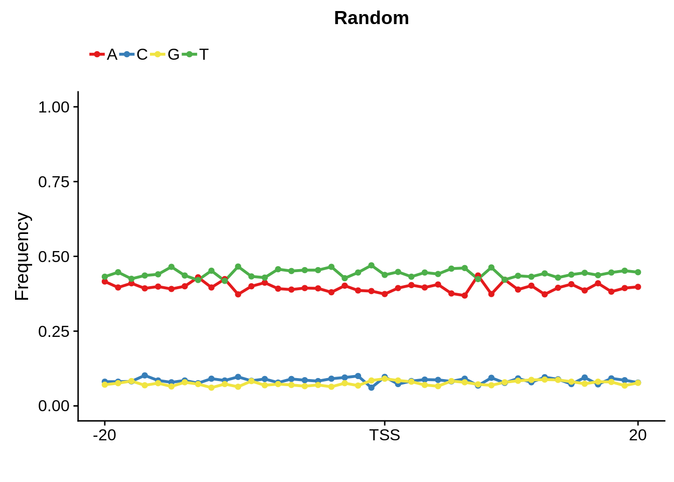
And we can see that the signal sort of goes away. However, there also wasn’t a very strong signal to begin with.
Tag clusters
The tag clusters represent high resolution TSSs that are enriched for the 5’ end of transcripts. Thus these TSS predictions are likely more accurate and less biased.
distance_to_add <- 500
# Use this function to filter tag clusters by total TPM
filter_tag_clusters <- function(tcs,tpm_threshold,width_threshold) {
broad_ftcs <- tcs %>%
tibble::as_tibble() %>%
dplyr::filter(as.numeric(tpm.dominant_ctss)>=tpm_threshold & interquantile_width >= width_threshold) %>%
dplyr::select(seqnames,dominant_ctss,strand,name) %>%
dplyr::distinct(seqnames,dominant_ctss,strand,name) %>%
dplyr::mutate(start=ifelse(strand=="+",
as.numeric(dominant_ctss)-(distance_to_add-1),
as.numeric(dominant_ctss)-(distance_to_add-1)),
end=ifelse(strand=="+",
as.numeric(dominant_ctss)+(distance_to_add+1),
as.numeric(dominant_ctss)+(distance_to_add+1))) %>%
GenomicRanges::GRanges()
sharp_ftcs <- tcs %>%
tibble::as_tibble() %>%
dplyr::filter(as.numeric(tpm.dominant_ctss)>=tpm_threshold & interquantile_width < width_threshold) %>%
dplyr::select(seqnames,dominant_ctss,strand,name) %>%
dplyr::distinct(seqnames,dominant_ctss,strand,name) %>%
dplyr::mutate(start=ifelse(strand=="+",
as.numeric(dominant_ctss)-(distance_to_add-1),
as.numeric(dominant_ctss)-(distance_to_add-1)),
end=ifelse(strand=="+",
as.numeric(dominant_ctss)+(distance_to_add+1),
as.numeric(dominant_ctss)+(distance_to_add+1))) %>%
GenomicRanges::GRanges()
return(list(sharp=sharp_ftcs,broad=broad_ftcs))
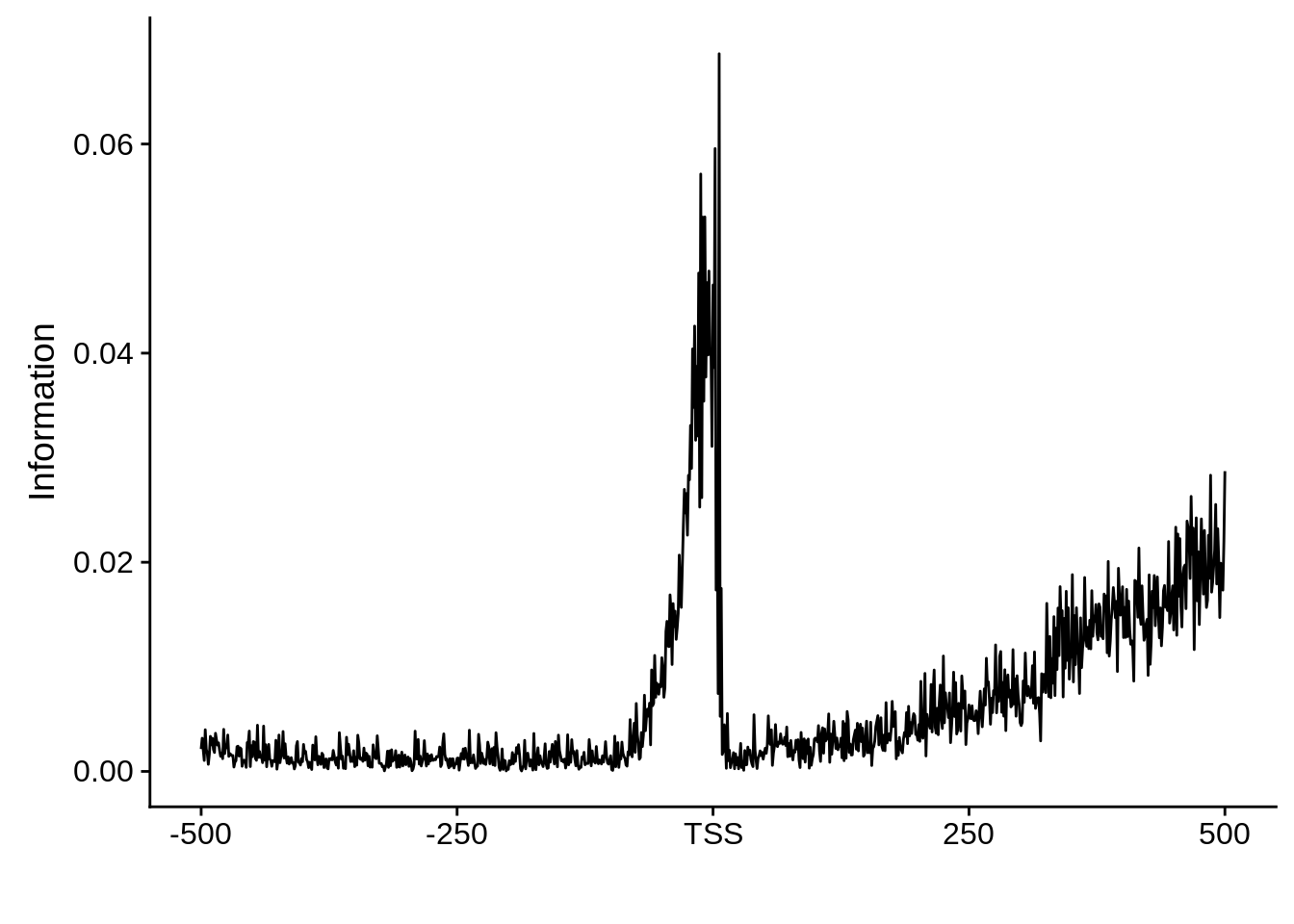
}Intergenic
# filter out clusters found in telomeres
tc_intergenic <- tc_intergenic[is.na(GenomicRanges::findOverlaps(tc_intergenic,telomeres,select="arbitrary"))]
ftcs <- filter_tag_clusters(tc_intergenic,5,15)
ftcssharppwm <- generate_pwm(ftcs$sharp)
ftcsbroadpwm <- generate_pwm(ftcs$broad)
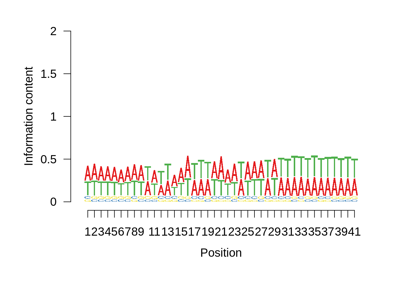
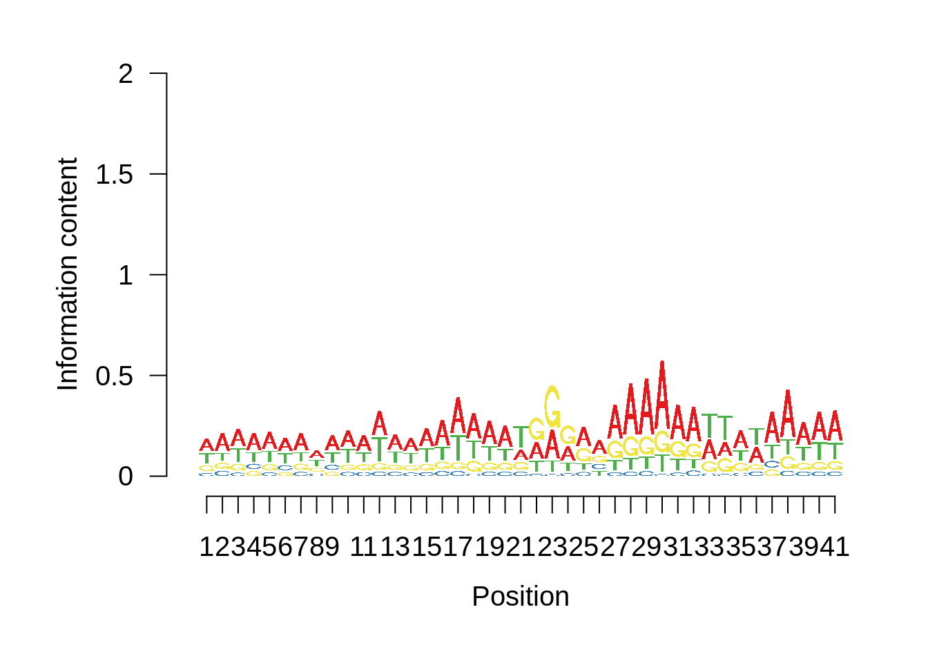
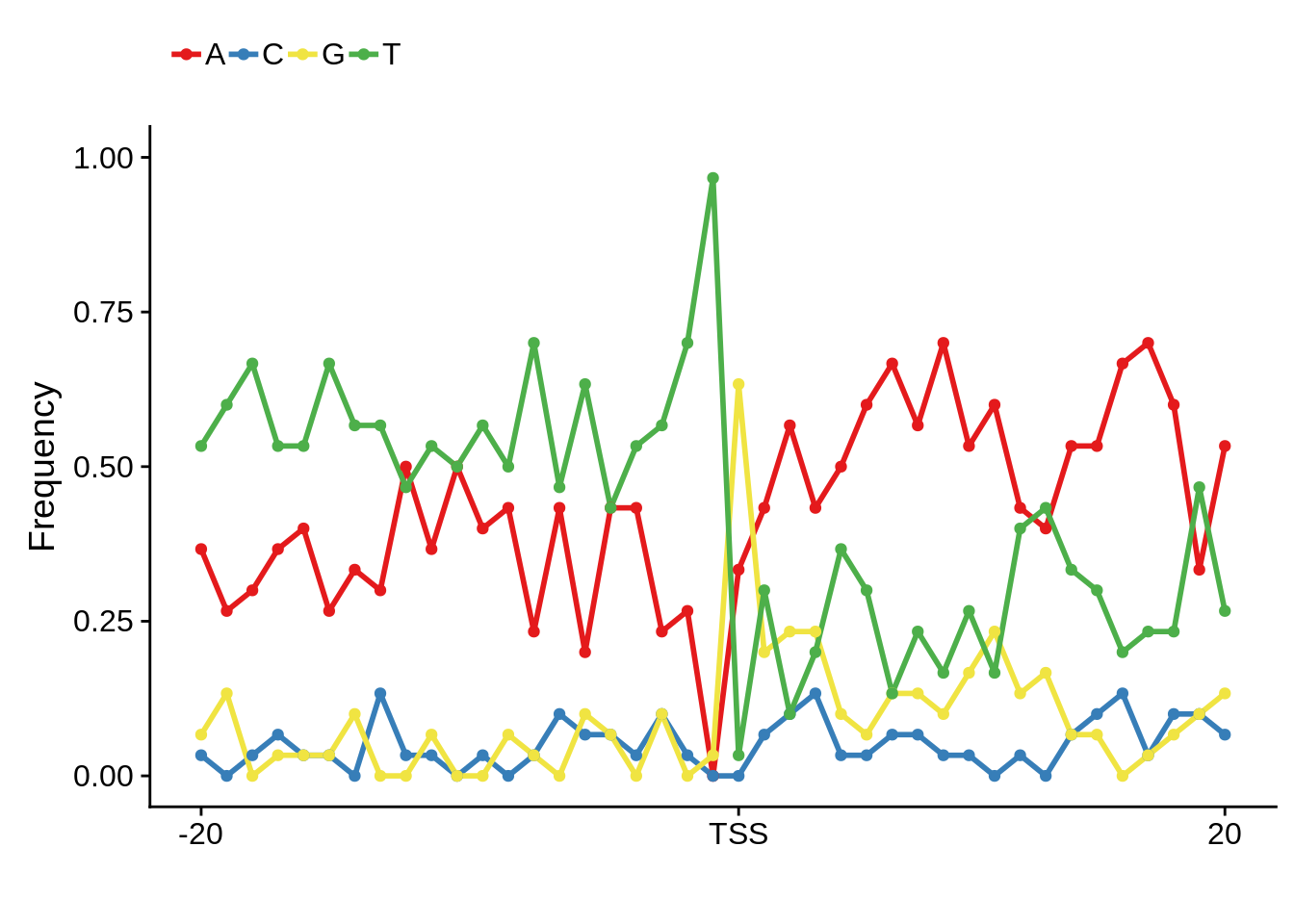
plot_frequencies(ftcssharppwm$pwm) + scale_x_continuous(limits=c(480,520),breaks=c(480,501,520),labels=c("-20","TSS","20"))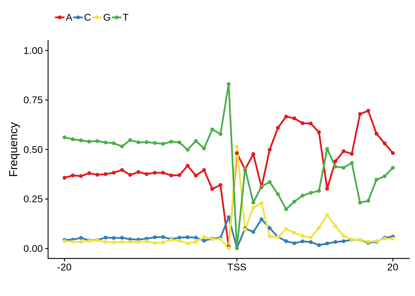
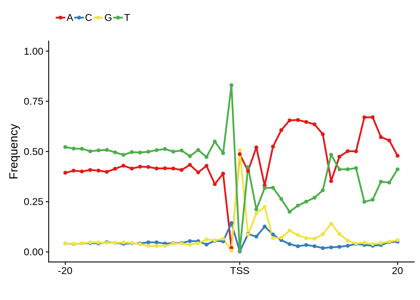
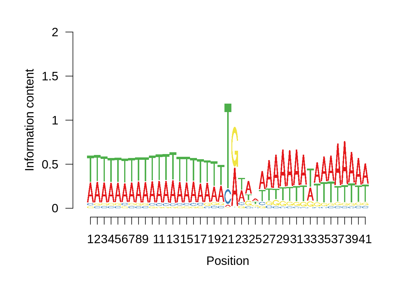
This is really interesting! Do we see the same thing if we look at the original TSO-predicted TSSs using a more biased approach? This method looked a certain distance upstream of every translation start site, used a 5 read threshold to discard positions that were not able to distinguish signal from noise, and designated the position with the greatest coverage upstream of an annotated protein-coding gene as the TSS.
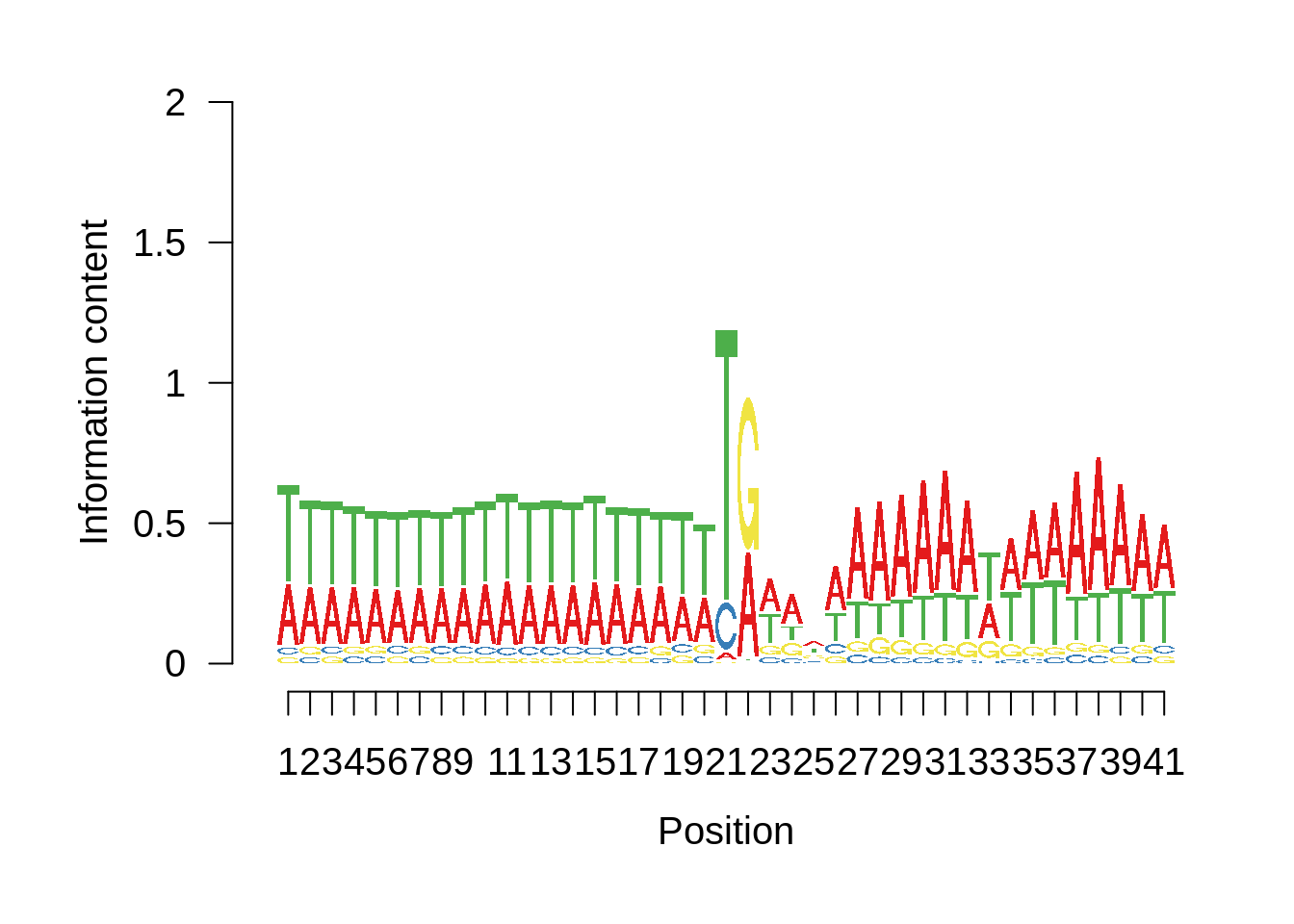
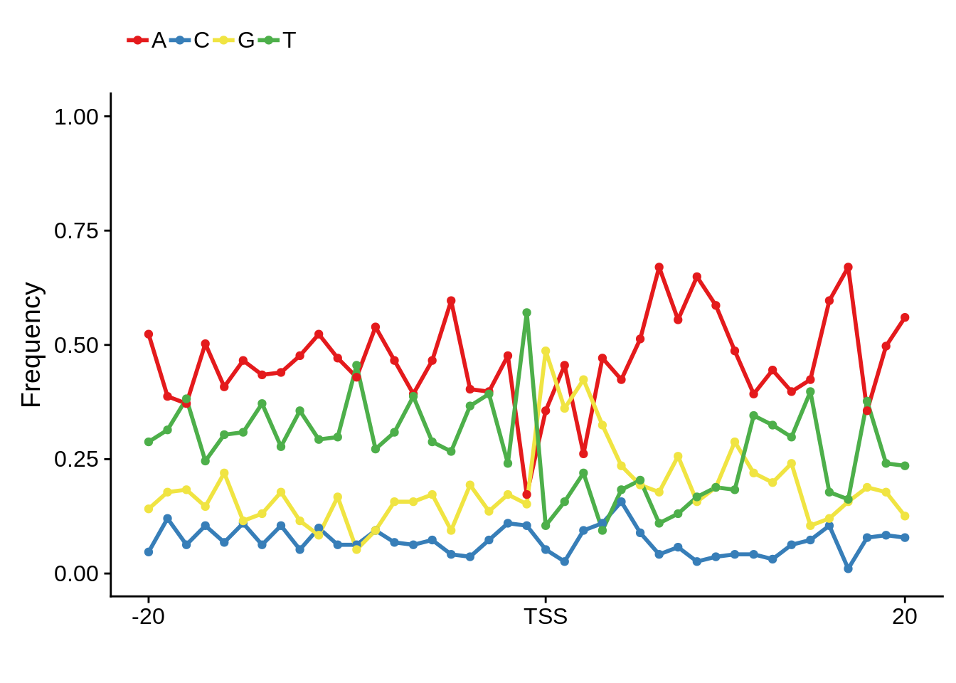
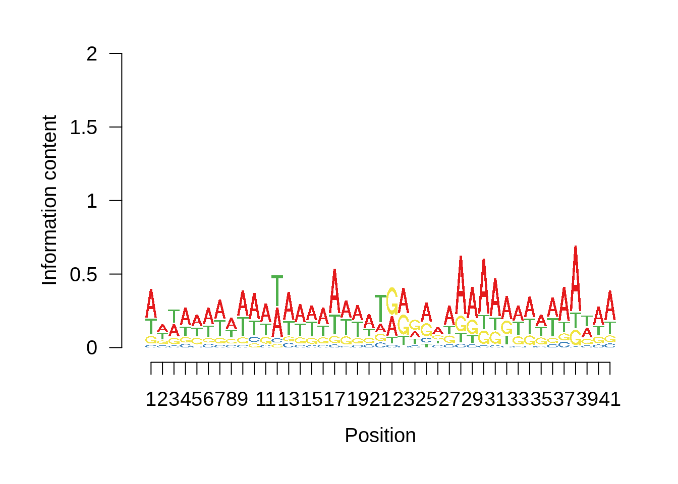
x3d7pwm <- generate_pwm(x3d7_tso)
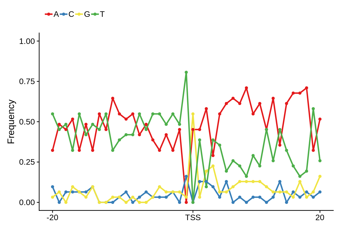
plot_frequencies(x3d7pwm$pwm) + scale_x_continuous(limits=c(480,520),breaks=c(480,501,520),labels=c("-20","TSS","20"))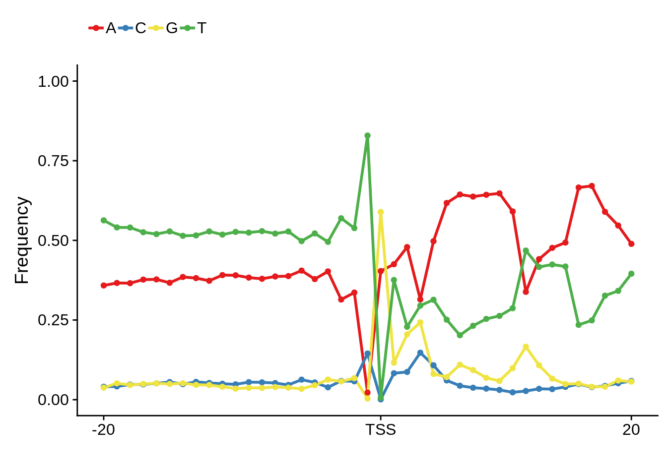
Exonic
fetcs <- filter_tag_clusters(tc_exonic,5,15)
fetcssharppwm <- generate_pwm(fetcs$sharp)
fetcsbroadpwm <- generate_pwm(fetcs$broad)
plot_frequencies(fetcssharppwm$pwm) + scale_x_continuous(limits=c(480,520),breaks=c(480,501,520),labels=c("-20","TSS","20"))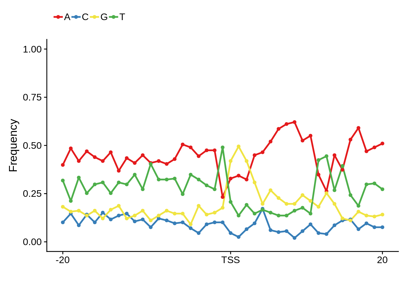
Nucleotide composition of sharp and broad promoters
In order to determine whether sharp and broad promoters are of significantly different nucleotide compositions, we first need to divide them up into sharp and broad promoters, then generate random sequences of similar length distributions, and compare the nucleotide content of the actual promoters to those of the randomly generated ones.
First let’s create random intergenic sequences:
# filter by total TPM
filter_promoter_clusters2 <- function(pcs,tpm_threshold) {
  # remove duplicates, add up total TPM, filter by threshold
  fpcs <- tibble::as_tibble(pcs) %>%
    dplyr::group_by(seqnames,start,strand,full_end,name) %>%
    dplyr::summarise(tpm=sum(as.numeric(tpm)),dominant_ctss=max(dominant_ctss)) %>%
    dplyr::filter(tpm >= tpm_threshold) %>%
    dplyr::ungroup() %>%
    dplyr::rename(end=full_end) %>%
    dplyr::mutate(end=as.numeric(end))
  return(fpcs)
}
# split by an arbitrary width and extract broad and sharp sequences
extract_cluster_seqs <- function(pcs, width) {
  # split them by promoter width
  broad_pcs <- GenomicRanges::GRanges(dplyr::filter(pcs, end-start >= width))
  sharp_pcs <- GenomicRanges::GRanges(dplyr::filter(pcs, end-start < width))
  # retrieve the sequences
  broad_seqs <- BSgenome::getSeq(BSgenome.Pfalciparum.PlasmoDB.v24,broad_pcs)
  sharp_seqs <- BSgenome::getSeq(BSgenome.Pfalciparum.PlasmoDB.v24,sharp_pcs)
  return(list(broad=broad_seqs,sharp=sharp_seqs))
}
# create random seqs to compare to
extract_random_seqs2 <- function(seqs,widths) {
  # start with the first sequence,
  # filter by width to avoid errors,
  # sample randomly from filtered sequences,
  # grab random interval that matches the length of the
  # promoter sequence
  fseqs       <- seqs[width(seqs) > widths[1]]
  rsample     <- sample(1:length(fseqs),size=1)
  rseq        <- fseqs[rsample][[1]]
  rstart      <- sample(x=1:(length(rseq)-widths[1]),size=1)
  random_seqs <- rseq[rstart:(rstart+widths[1]-1)]
  # do this for all sequences
  for (i in 2:length(widths)) {
    fseqs       <- seqs[width(seqs) > widths[i]]
    rsample     <- sample(1:length(fseqs),size=1)
    rseq        <- fseqs[rsample][[1]]
    rstart      <- sample(x=1:(length(rseq)-widths[i]-1),size=1)
    random_seqs <- unlist(Biostrings::DNAStringSetList(
      Biostrings::DNAStringSet(random_seqs),
      Biostrings::DNAStringSet(rseq[rstart:(rstart+widths[i]-1)])))
  }
  return(random_seqs)
}

# calculate promoter cluster nucleotide frequencies
calculate_frequencies <- function(cluster_seqs,random_seqs) {
  # calculate nucleotide frequencies for broad promoters
  clengths <- BSgenome::width(cluster_seqs$broad)
  cfreqs   <- BSgenome::oligonucleotideFrequency(x=cluster_seqs$broad,width=1,step=1,as.prob=TRUE)
  rlengths <- BSgenome::width(random_seqs$broad)
  rfreqs   <- BSgenome::oligonucleotideFrequency(x=random_seqs$broad,width=1,step=1,as.prob=TRUE)
  cluster_broad_tibble <- tibble::tibble(length=clengths,
                                 AT=(cfreqs[,1]+cfreqs[,4]),
                                 GC=(cfreqs[,2]+cfreqs[,3]),
                                 shape="broad") %>%
    dplyr::select(length,AT,GC,shape)
  random_broad_tibble <- tibble::tibble(length=rlengths,
                                 AT=(rfreqs[,1]+rfreqs[,4]),
                                 GC=(rfreqs[,2]+rfreqs[,3]),
                                 shape="broad") %>%
    dplyr::select(length,AT,GC,shape)
  # calculate nucleotide frequencies for sharp promoters
  clengths <- BSgenome::width(cluster_seqs$sharp)
  cfreqs   <- BSgenome::oligonucleotideFrequency(x=cluster_seqs$sharp,width=1,step=1,as.prob=TRUE)
  rlengths <- BSgenome::width(random_seqs$sharp)
  rfreqs   <- BSgenome::oligonucleotideFrequency(x=random_seqs$sharp,width=1,step=1,as.prob=TRUE)
  cluster_sharp_tibble <- tibble::tibble(length=clengths,
                                 AT=(cfreqs[,1]+cfreqs[,4]),
                                 GC=(cfreqs[,2]+cfreqs[,3]),
                                 shape="sharp") %>%
    dplyr::select(length,AT,GC,shape)
  random_sharp_tibble <- tibble::tibble(length=rlengths,
                                 AT=(rfreqs[,1]+rfreqs[,4]),
                                 GC=(rfreqs[,2]+rfreqs[,3]),
                                 shape="sharp") %>%
    dplyr::select(length,AT,GC,shape)
  # combine into one tibble
  cluster_shape_tibble <- dplyr::bind_rows(cluster_broad_tibble,cluster_sharp_tibble)
  random_shape_tibble <- dplyr::bind_rows(random_broad_tibble,random_sharp_tibble)
  return(list(cluster_shape_tibble=cluster_shape_tibble,random_shape_tibble=random_shape_tibble))
}

# generate shape nucleotide frequency
generate_shape_frequencies <- function(pcs,seqs,filter_threshold,split_width,freq_fun) {
  # filter by TPM threshold
  fpcs <- filter_promoter_clusters2(pcs,filter_threshold)
  # split by arbitrary width
  cluster_seqs <- extract_cluster_seqs(fpcs,split_width)
  # generate random promoter clusters of similar widths
  random_seqs <- list(broad=extract_random_seqs2(seqs=seqs,widths=width(cluster_seqs$broad)),
                      sharp=extract_random_seqs2(seqs=seqs,widths=width(cluster_seqs$sharp))
                  )
  # normalize by nucleotide frequencies of random sequences
  shape_tibble <- do.call(freq_fun,list(cluster_seqs=cluster_seqs,random_seqs=list(broad=random_seqs$broad,sharp=random_seqs$sharp)))
  return(shape_tibble)
}
First we can look at the nucleotide composition for intergenic promoters:
# first we can do this for intergenic sequences
genes      <- rtracklayer::import.gff3("../data/annotations/genes_nuclear_3D7_v24.gff")
telomeres  <- rtracklayer::import.gff3("../data/annotations/Pf3D7_v3_subtelomeres.gff")
intergenic <- GenomicRanges::gaps(genes)
intergenic <- intergenic[is.na(GenomicRanges::findOverlaps(intergenic,telomeres,select="arbitrary"))]
intergenic_seqs <- BSgenome::getSeq(BSgenome.Pfalciparum.PlasmoDB.v24,intergenic)
Now we’ll generate the frequencies without normalization:
shape_tibble <- generate_shape_frequencies(pcs=pc_intergenic,
                                           seqs=intergenic_seqs,
                                           filter_threshold=5,
                                           split_width=15,
                                           freq_fun=calculate_frequencies)

readr::write_tsv(x=shape_tibble$cluster_shape_tibble,path="../output/promoter_architecture/cluster_shape_frequencies.tsv")
readr::write_tsv(x=shape_tibble$random_shape_tibble,path="../output/promoter_architecture/random_shape_frequencies.tsv")
But we’ll also generate them within normalization and repeat the random sampling 100 times:
Now we can look at some plots of the frequencies:
# read in precalculated frequencies
cluster_shape_tibble <- readr::read_tsv(file="../output/promoter_architecture/cluster_shape_frequencies.tsv")
random_shape_tibble <- readr::read_tsv(file="../output/promoter_architecture/random_shape_frequencies.tsv")
# plot nucleotide frequencies
g <- cluster_shape_tibble %>% ggplot(aes(x=shape,y=GC)) + geom_boxplot()
print(g)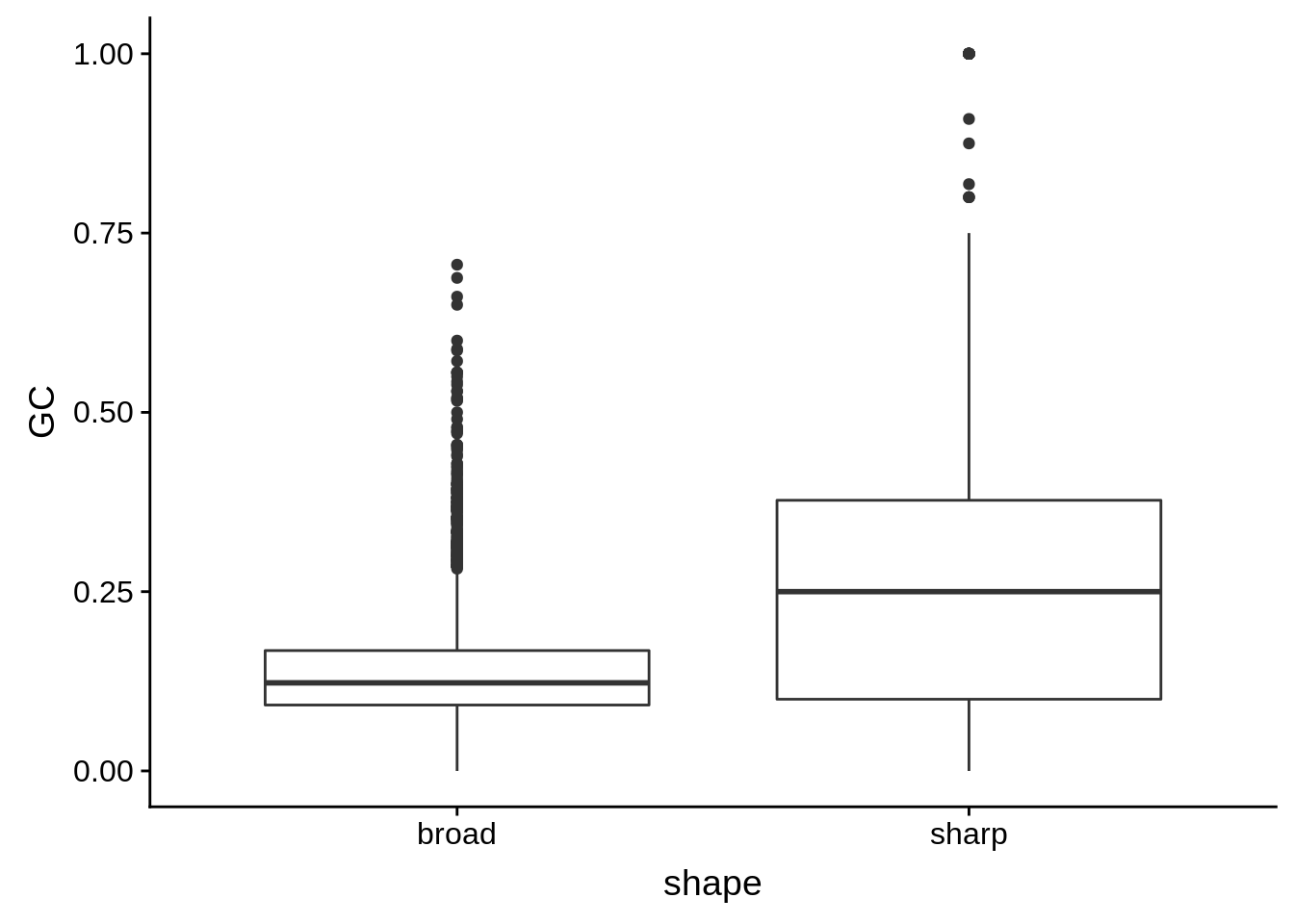
g <- cluster_shape_tibble %>% ggplot(aes(x=GC,color=shape)) + geom_line(stat="density",size=1)
print(g)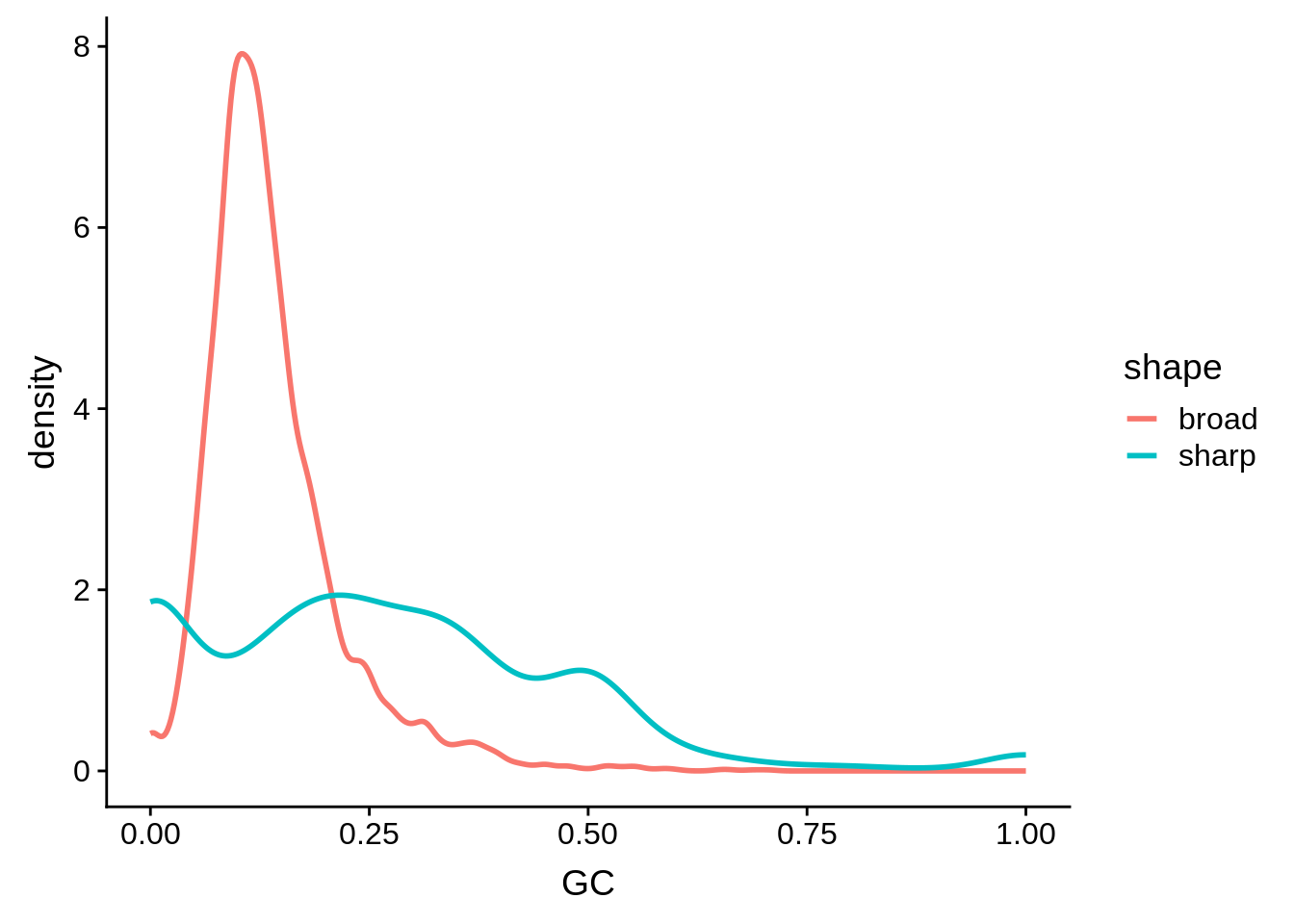
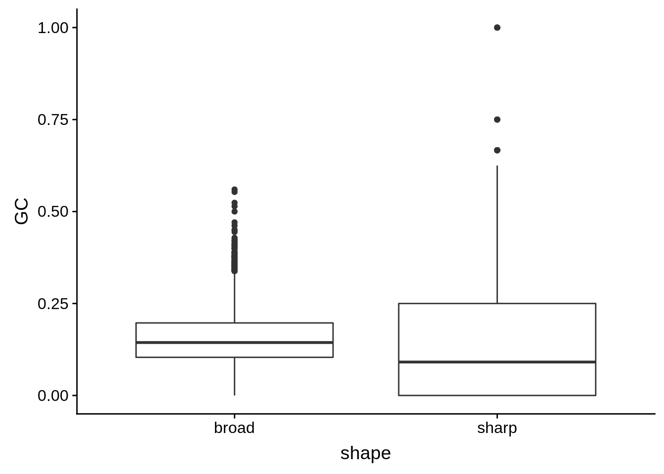
g <- random_shape_tibble %>% ggplot(aes(x=GC,color=shape)) + geom_line(stat="density",size=1)
print(g)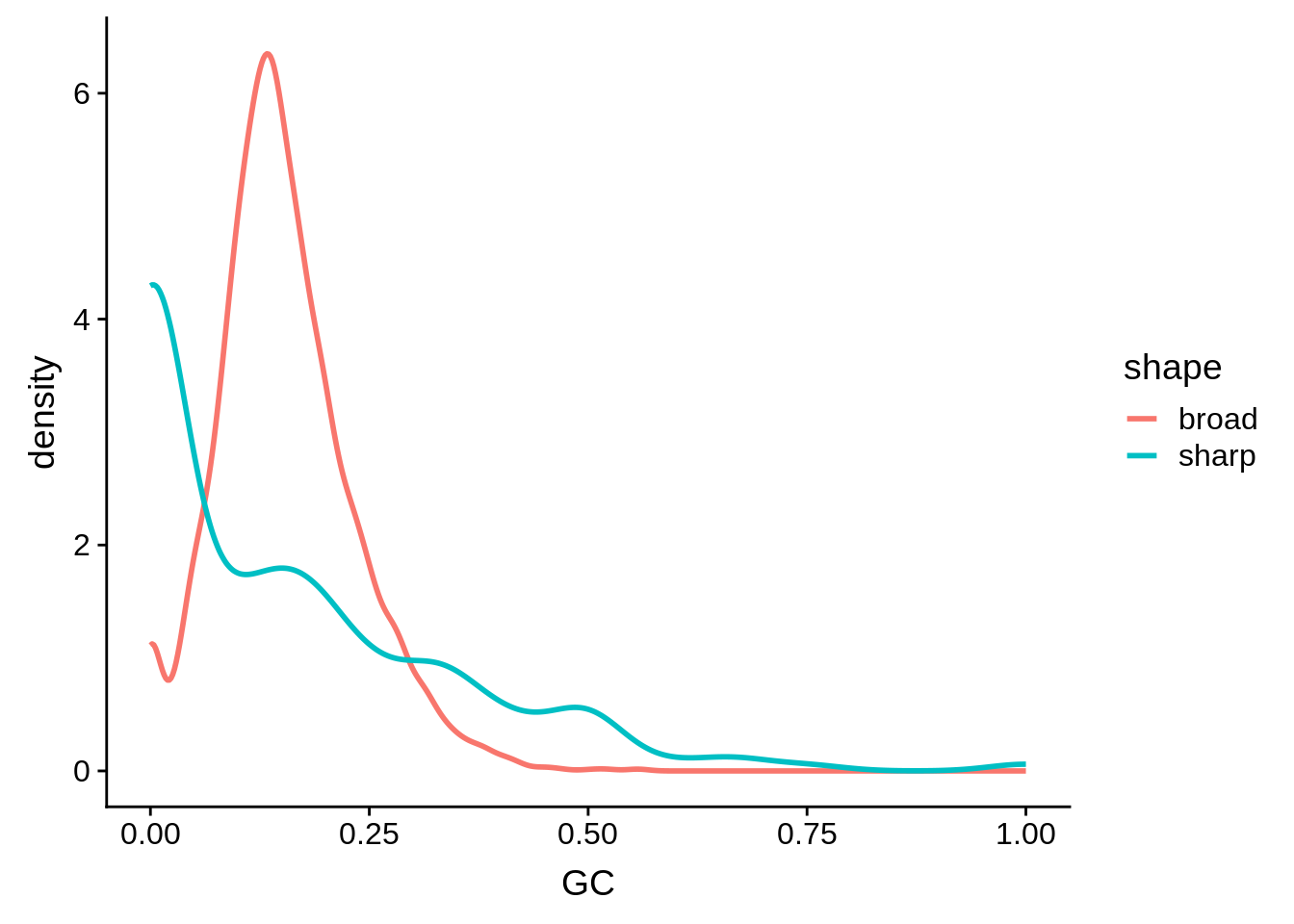
Manuscript numbers
How many tag clusters?
[1] 17375[1] 1175[1] 186How many promoter clusters?
[1] 20879[1] 1253[1] 197Is there anything functionally enriched in the set of genes with many TSSs?
core_genes <- readr::read_tsv("../data/gene_lists/core_pf3d7_genes.txt",col_names=F)$X1
out <- tc_intergenic %>%
  tibble::as_tibble() %>%
  dplyr::group_by(seqnames,start,end,name,tp) %>%
  dplyr::filter(as.numeric(tpm.dominant_ctss) >= 2) %>%
  dplyr::group_by(name,tp) %>%
  dplyr::summarise(n=n()) %>%
  dplyr::filter(n >= 5 & name %in% core_genes) %$%
  unique(name)

readr::write_lines(x=out,path="../output/promoter_architecture/5_annotated_tcs.txt")How many broad/sharp promoters per timepoint?
# abundance estimates
x3d7_abund <- readRDS("../output/neighboring_genes/gene_reduced_3d7_abund.rds")
xhb3_abund <- readRDS("../output/neighboring_genes/gene_reduced_hb3_abund.rds")
xit_abund  <- readRDS("../output/neighboring_genes/gene_reduced_it_abund.rds")

pcg <- tibble::as_tibble(rtracklayer::import.gff3("../data/annotations/PF3D7_codinggenes_for_bedtools.gff"))$ID
get_filtered_ids <- function(abund,tpm_threshold) {
  fabund <- abund %>%
    dplyr::group_by(gene_id) %>%
    dplyr::summarise(f=sum(TPM>=tpm_threshold)) %>%
    dplyr::ungroup() %>%
    dplyr::filter(f>0 & gene_id %in% pcg)
  return(fabund$gene_id)
}

fx3d7 <- get_filtered_ids(x3d7_abund,5)
fxhb3 <- get_filtered_ids(xhb3_abund,5)
fxit  <- get_filtered_ids(xit_abund,5)

intertags <- dplyr::inner_join(as_tibble(tc_intergenic) %>% dplyr::mutate(tp=as.integer(tp)),x3d7_abund,by=c("name" = "gene_id","tp"))

intertags$type <- ifelse(intertags$interquantile_width >= 15, "broad", "sharp")
intertags %>%
  dplyr::filter(as.numeric(tpm.dominant_ctss) >= 2 & abs(as.numeric(anno_start) - as.numeric(dominant_ctss)) <= 2500) %>%
  ggplot(aes(x=tp,fill=type)) +
  geom_bar(colour="black",size=1.0) +
  scale_fill_brewer(palette="Greys") +
  ylab("Frequency") +
  xlab("Timepoint") +
  theme(axis.text=element_text(size=18),
        axis.title=element_text(size=20,face="bold"),
        axis.line.x=element_line(colour="black",size=1.5),
        axis.ticks.x=element_line(colour="black",size=1.5),
        axis.line.y=element_line(colour="black",size=1.5),
        axis.ticks.y=element_line(colour="black",size=1.5),
        legend.text=element_text(size=16),
        legend.title=element_blank()) +
  labs("") +
  scale_x_continuous(breaks=c(1,2,3,4,5,6,7))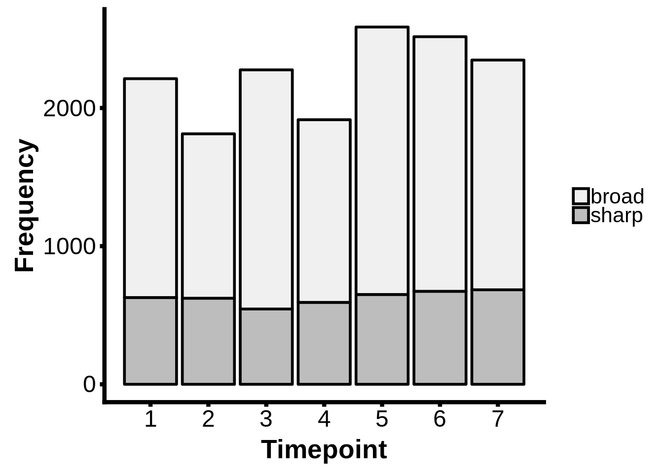
Is there actually an expression difference between genes annotated with sharp and genes annotated with broad PCs?
s <- dplyr::filter(intertags, type=="sharp")
b <- dplyr::filter(intertags, type=="broad")

sabund <- x3d7_abund %>% dplyr::filter(gene_id %in% s$name) %>% dplyr::mutate(type="sharp")
babund <- x3d7_abund %>% dplyr::filter(gene_id %in% b$name) %>% dplyr::mutate(type="broad")

nabund <- dplyr::bind_rows(sabund,babund)

nabund %>% dplyr::filter(strain == "3d7") %>%
  ggplot(aes(x=type,y=log2(TPM+1))) +
  geom_boxplot() +
  facet_grid(~tp) +
  ylab("Log2 TPM") +
  xlab("")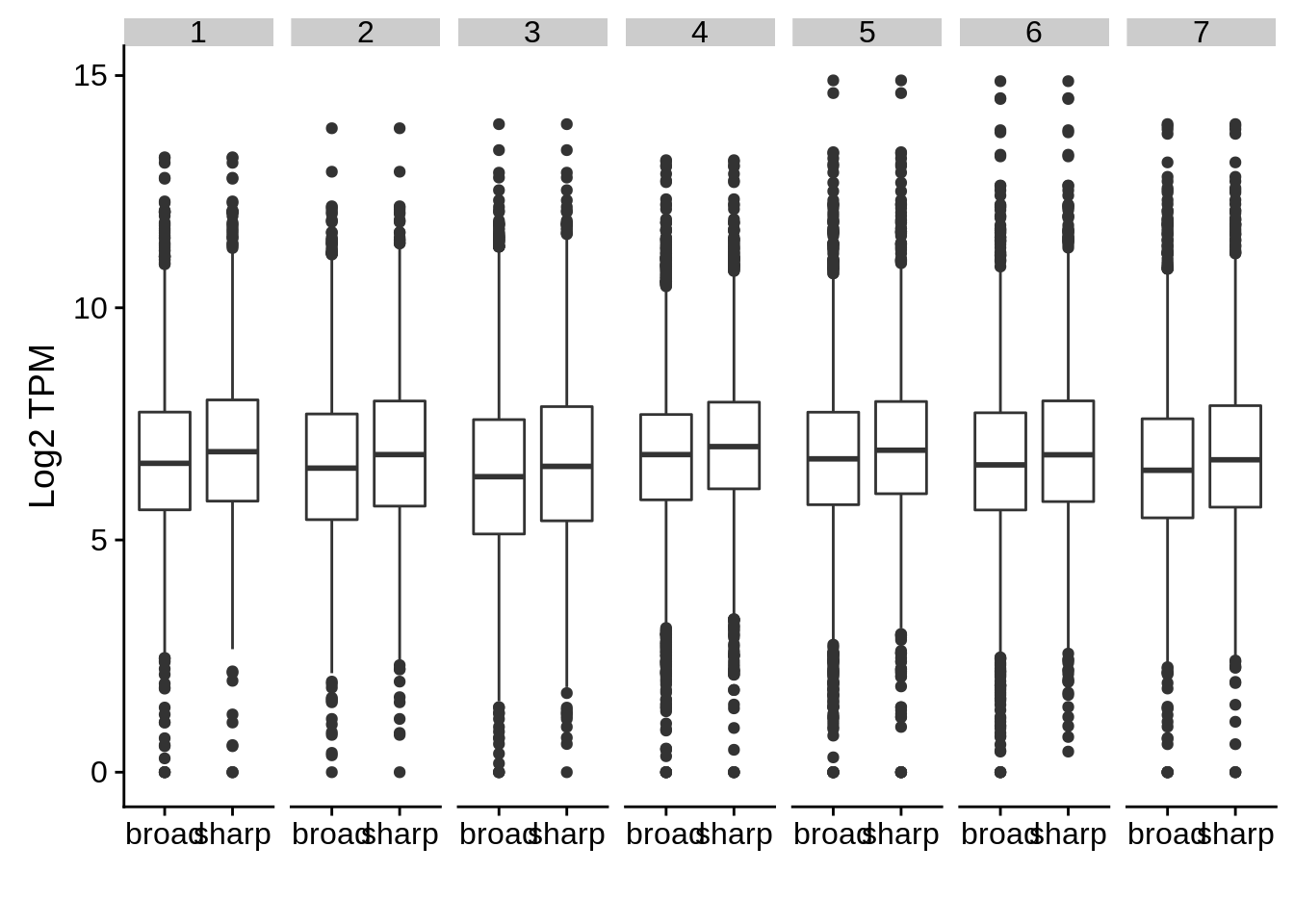
for (i in c(1,2,3,4,5,6,7)) {
  h1 <- sabund %>% dplyr::filter(tp==i)
  h2 <- babund %>% dplyr::filter(tp==i)
  print(t.test(log2(h1$TPM+1),log2(h2$TPM+1)))
}
    Welch Two Sample t-test

data:  log2(h1$TPM + 1) and log2(h2$TPM + 1)
t = 5.6435, df = 5248.1, p-value = 1.754e-08
alternative hypothesis: true difference in means is not equal to 0
95 percent confidence interval:
 0.1641908 0.3389816
sample estimates:
mean of x mean of y
 6.996609  6.745023


    Welch Two Sample t-test

data:  log2(h1$TPM + 1) and log2(h2$TPM + 1)
t = 5.9559, df = 5250.9, p-value = 2.755e-09
alternative hypothesis: true difference in means is not equal to 0
95 percent confidence interval:
 0.1874511 0.3714007
sample estimates:
mean of x mean of y
 6.905630  6.626204


    Welch Two Sample t-test

data:  log2(h1$TPM + 1) and log2(h2$TPM + 1)
t = 5.4934, df = 5245.1, p-value = 4.129e-08
alternative hypothesis: true difference in means is not equal to 0
95 percent confidence interval:
 0.181309 0.382524
sample estimates:
mean of x mean of y
 6.701573  6.419657


    Welch Two Sample t-test

data:  log2(h1$TPM + 1) and log2(h2$TPM + 1)
t = 5.6408, df = 5270.8, p-value = 1.781e-08
alternative hypothesis: true difference in means is not equal to 0
95 percent confidence interval:
 0.1704441 0.3520227
sample estimates:
mean of x mean of y
 7.060800  6.799567


    Welch Two Sample t-test

data:  log2(h1$TPM + 1) and log2(h2$TPM + 1)
t = 5.1856, df = 5253.1, p-value = 2.234e-07
alternative hypothesis: true difference in means is not equal to 0
95 percent confidence interval:
 0.1489161 0.3299533
sample estimates:
mean of x mean of y
 6.999417  6.759982


    Welch Two Sample t-test

data:  log2(h1$TPM + 1) and log2(h2$TPM + 1)
t = 5.3448, df = 5270.1, p-value = 9.434e-08
alternative hypothesis: true difference in means is not equal to 0
95 percent confidence interval:
 0.1551941 0.3349887
sample estimates:
mean of x mean of y
 6.937661  6.692569


    Welch Two Sample t-test

data:  log2(h1$TPM + 1) and log2(h2$TPM + 1)
t = 5.4173, df = 5228.2, p-value = 6.321e-08
alternative hypothesis: true difference in means is not equal to 0
95 percent confidence interval:
 0.1609049 0.3434045
sample estimates:
mean of x mean of y
 6.856455  6.604300
Is there anything significant about gene annotated with shifting TSSs?
Session Information
R version 3.5.0 (2018-04-23)
Platform: x86_64-pc-linux-gnu (64-bit)
Running under: Gentoo/Linux

Matrix products: default
BLAS: /usr/local/lib64/R/lib/libRblas.so
LAPACK: /usr/local/lib64/R/lib/libRlapack.so

locale:
 [1] LC_CTYPE=en_US.UTF-8       LC_NUMERIC=C
 [3] LC_TIME=en_US.UTF-8        LC_COLLATE=en_US.UTF-8
 [5] LC_MONETARY=en_US.UTF-8    LC_MESSAGES=en_US.UTF-8
 [7] LC_PAPER=en_US.UTF-8       LC_NAME=C
 [9] LC_ADDRESS=C               LC_TELEPHONE=C
[11] LC_MEASUREMENT=en_US.UTF-8 LC_IDENTIFICATION=C

attached base packages:
[1] parallel  stats4    stats     graphics  grDevices utils     datasets
[8] methods   base

other attached packages:
 [1] bindrcpp_0.2.2
 [2] BSgenome.Pfalciparum.PlasmoDB.v24_1.0
 [3] BSgenome_1.48.0
 [4] rtracklayer_1.40.6
 [5] Biostrings_2.48.0
 [6] XVector_0.20.0
 [7] GenomicRanges_1.32.6
 [8] GenomeInfoDb_1.16.0
 [9] org.Pf.plasmo.db_3.6.0
[10] AnnotationDbi_1.42.1
[11] IRanges_2.14.10
[12] S4Vectors_0.18.3
[13] Biobase_2.40.0
[14] BiocGenerics_0.26.0
[15] scales_1.0.0
[16] cowplot_0.9.3
[17] magrittr_1.5
[18] forcats_0.3.0
[19] stringr_1.3.1
[20] dplyr_0.7.6
[21] purrr_0.2.5
[22] readr_1.1.1
[23] tidyr_0.8.1
[24] tibble_1.4.2
[25] ggplot2_3.0.0
[26] tidyverse_1.2.1

loaded via a namespace (and not attached):
 [1] nlme_3.1-137                bitops_1.0-6
 [3] matrixStats_0.54.0          lubridate_1.7.4
 [5] bit64_0.9-7                 RColorBrewer_1.1-2
 [7] httr_1.3.1                  rprojroot_1.3-2
 [9] tools_3.5.0                 backports_1.1.2
[11] R6_2.2.2                    seqLogo_1.34.0
[13] DBI_1.0.0                   lazyeval_0.2.1
[15] colorspace_1.3-2            withr_2.1.2
[17] tidyselect_0.2.4            bit_1.1-14
[19] compiler_3.5.0              git2r_0.23.0
[21] cli_1.0.0                   rvest_0.3.2
[23] xml2_1.2.0                  DelayedArray_0.6.5
[25] labeling_0.3                digest_0.6.15
[27] Rsamtools_1.32.3            rmarkdown_1.10
[29] R.utils_2.6.0               pkgconfig_2.0.2
[31] htmltools_0.3.6             rlang_0.2.2
[33] readxl_1.1.0                rstudioapi_0.7
[35] RSQLite_2.1.1               bindr_0.1.1
[37] jsonlite_1.5                BiocParallel_1.14.2
[39] R.oo_1.22.0                 RCurl_1.95-4.11
[41] GenomeInfoDbData_1.1.0      Matrix_1.2-14
[43] Rcpp_0.12.18                munsell_0.5.0
[45] R.methodsS3_1.7.1           stringi_1.2.4
[47] yaml_2.2.0                  SummarizedExperiment_1.10.1
[49] zlibbioc_1.26.0             plyr_1.8.4
[51] grid_3.5.0                  blob_1.1.1
[53] crayon_1.3.4                lattice_0.20-35
[55] haven_1.1.2                 hms_0.4.2
[57] knitr_1.20                  pillar_1.3.0
[59] reshape2_1.4.3              XML_3.98-1.16
[61] glue_1.3.0                  evaluate_0.11
[63] modelr_0.1.2                cellranger_1.1.0
[65] gtable_0.2.0                assertthat_0.2.0
[67] broom_0.5.0                 GenomicAlignments_1.16.0
[69] memoise_1.1.0               workflowr_1.1.1
This R Markdown site was created with workflowr