
Data Analysis Examples
Meetup #4
Data Analysis Examples
- YouTube Video Ranking
- Bayesian Rankings vs ML Rankings
- Bayesian Rankings vs ML Rankings
- Caribbean Crime Forecasting
- Hierarchical Modeling
- Gaussian Processes
- Paint By Numbers
- Mixture Models
- Infinite Mixture Models
- Putting it all together
Ranking YouTube Videos
- Collect some data
- Determine the best ones by looking at which are "liked" with the highest probability
Done. Maybe?
Get Some Data
videos = get_videos('office+pranks', 50)
stats = get_statistics(videos)[['title', 'likeCount', 'dislikeCount']]
stats.head(15)
Rank by likeCount Ratio
stats['totalVotes'] = stats['likeCount'] + stats['dislikeCount']
stats['p'] = stats['likeCount'].astype(np.float64) / stats['totalVotes']
stats.sort(['p', 'totalVotes'], ascending=False).head(25)
Video Ranking Model
What we're really doing:
$$p_i \text{ = Probability that an individual viewer will like video }i\text{,}$$$$L_i \text{ = # of Likes for video }i\text{,}$$$$D_i \text{ = # of Dislikes for video }i$$$$n_i = L_i + D_i$$Model Realistic? Sort of.
Maximum Likelihood Estimate for $p_i$ = $\frac{L_i}{n_i}$
Good estimate? Yea, but not when the sample size (i.e. $n_i$) is small (e.g. 1/1, 2/2, 0/1)
How can we model the probability of a like but somehow account for sample size?
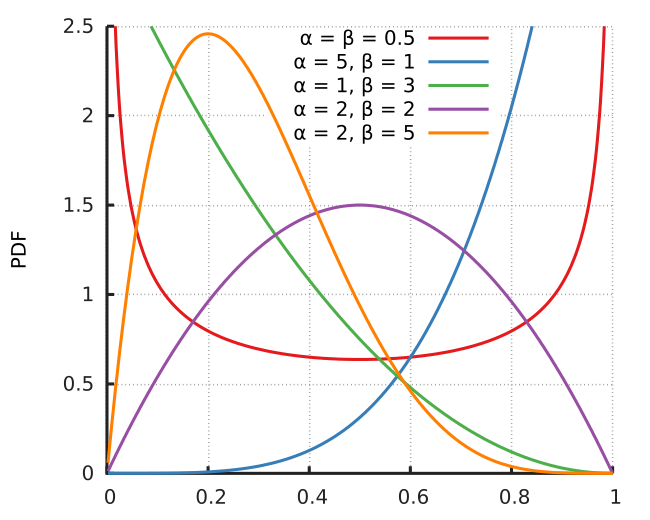
The Beta Distribution
It's only defined on 0 to 1 and has two parameters, plenty enough to manipulate the shape to be what we want.
Probability Density Function: $$ p(x) = \frac{x^{\alpha - 1}(1 - x)^{\beta - 1}}{B(\alpha, \beta)},$$ where $B$ is the Beta Function
Making up a Solution
Let's just say this because why not:
- $\alpha$ parameter in $B$ distribution = # video likes
- $\beta$ parameter in $B$ distribution = # video dislikes
What do these distributions look like for videos with the same like / dislike ratio?
Say 4 videos had the following stats:
| Video | Likes | Dislikes | Ratio |
|---|---|---|---|
| 1 | 9 | 3 | 9/3 = 3 |
| 2 | 15 | 5 | 15/5 = 3 |
| 3 | 48 | 16 | 48/16 = 3 |
| 4 | 600 | 200 | 600/200 = 3 |
%%R -w 800 -h 400 -u px
n <- 10000
rbind(
data.frame(name='Video 1 - Beta(9, 3)', value=rbeta(n,6,2)),
data.frame(name='Video 2 - Beta(15, 5)', value=rbeta(n,15,5)),
data.frame(name='Video 3 - Beta(48, 16)', value=rbeta(n,48,16)),
data.frame(name='Video 4 - Beta(600, 200)', value=rbeta(n,600,200))
) %>%
ggplot(aes(x=value)) + geom_density() + xlab('p') +
facet_wrap(~name, ncol=2, scale="free_y") +
ggtitle('Beta Distribution for Each Video') +
theme_bw()

%%R -w 800 -h 400 -u px
n <- 10000
rbind(
data.frame(name='Video 1 - Beta(9, 3)', value=rbeta(n,9,3), lo=qbeta(.05,9,3), mean=9/12),
data.frame(name='Video 2 - Beta(15, 5)', value=rbeta(n,15,5), lo=qbeta(.05,15,5), mean=15/20),
data.frame(name='Video 3 - Beta(48, 16)', value=rbeta(n,48,16), lo=qbeta(.05,48,16), mean=48/64),
data.frame(name='Video 4 - Beta(600, 200)', value=rbeta(n,600,200), lo=qbeta(.05,600,200), mean=600/800)
) %>%
ggplot(aes(x=value)) + geom_density() + xlab('p') +
facet_wrap(~name, ncol=2, scale="free_y") +
ggtitle('Beta Distribution for Each Video') +
geom_vline(aes(xintercept=lo), color='red', linetype=2) +
geom_vline(aes(xintercept=mean), color='black') +
theme_bw()

How to get there?
BEFORE we see any data, let's say we estimate $p_i$ to be something flat like this:
ax = pd.Series(np.repeat(1, 100), np.linspace(0, 1, 100)).plot()
ax.set_xlabel('$p_i$')
ax.set_ylabel('$Density$')
ax.set_title('Beta(1, 1) Distribution')

Bayes Theorem
Given a prior belief in $p_i$ AND some data $D$, what should be our new belief as to what $p_i$ is?
Luckily there are some rules that will help:
In English:
$$= \frac{Pr( \text{X likes and Y dislikes given a value for }p_i) \cdot Pr(p_i\text{in the first place})}{\text{the sum of all possible values for the numerator}} $$
The bayesian lingo:
Example
- Say our data, $D$, was 2 likes and 1 dislike
- Also say the we want to calculate an approximation to the posterior for $p \in [.1, .5, .9]$
| p | Pr(D|p) | Pr(p) | Pr(D|p) * Pr(p) |
|---|---|---|---|
| .1 | 3 * .1^2 * (1-.1) = 0.027 | 1 | 0.027 |
| .5 | 3 * .5^2 * (1-.5) = 0.375 | 1 | 0.375 |
| .9 | 3 * .9^2 * (1-.9) = 0.243 | 1 | 0.243 |
marginal - The sum of all "likelihood * prior" values = 0.027 + 0.375 + 0.243 = 0.645
Posterior Estimate
Divide last column above by sum (over same column) to get posterior estimate:
| p | Pr(D|p) * Pr(p) / marginal | Posterior: Pr(p|D) |
|---|---|---|
| .1 | 0.027 / 0.645 | 0.042 |
| .5 | 0.375 / 0.645 | 0.581 |
| .9 | 0.243 / 0.645 | 0.377 |
Back to Theory
The "likelihood" or $Pr(D|p)$ above is technically from a binomial distribution
The mass function of this distribution is:
$$P(k, n) \sim \textstyle {n \choose k}\, p^k (1-p)^{n-k}$$
- $k$ is the number of likes in our case
- $n$ is the number of likes + number of dislikes (ie votes)
- $p$ is a current estimate for the actual $p_i$ (ie the probability of getting a like)
Recall the "prior" was from a Beta distribution with density function:
$$P(p) = p^{\alpha - 1}(1 - p)^{\beta - 1}/B(\alpha, \beta)$$
- $p$ is probability of getting a like
- Our prior used so far was $Beta(1, 1)$ but in general, you can have any prior like $Beta(\alpha, \beta)$
Posteriors
- The posterior actually looks like this then:
- Given the above things, plugging it all together gives (but leaving out the sum/integral on the bottom):
The Punchline
Through algrebra and magic, the posterior actually reduces to another BETA distribution. The final form is:
$$ Pr(p_i|L_i,D_i,n_i) = \text{Beta}(\alpha + L_i, \beta + D_i)$$
If our prior was uniform (ie Beta(1, 1)), what is the distribution of $p_i$ if a video has 5 likes and 2 dislikes?
$$ p_1 \sim \text{Beta}(1 + 5, 1 + 2) = \text{Beta}(6, 3)$$
And for one with 50 likes and 20 dislikes?
$$ p_2 \sim \text{Beta}(1 + 50, 1 + 20) = \text{Beta}(51, 21)$$
%%R -u px -h 400 -w 1200
data.frame(x=seq(0, 1, .01)) %>%
mutate('5.likes'=dbeta(x, 6, 3), '50.likes'=dbeta(x, 51, 21)) %>%
melt(id.vars='x') %>% ggplot(aes(x=x, y=value, color=variable)) + geom_line() + theme_bw()

Applying Bayesian Rank to Data
- Apply the model above to our YouTube videos and see how that changes the list:
from scipy.stats import beta
print('Top 10 Videos by Bayesian Rank:')
videos['bayes.p'] = videos.apply(lambda x: beta.ppf(.5, x['likes'] + 1, x['dislikes'] + 1), axis=1)
videos.sort(['bayes.p', 'n'], ascending=False).head(10)
print('Top 10 Videos by Maximum Likelihood Rank:')
videos.sort(['p', 'n'], ascending=False).head(10)
%%R -u px -w 800 -h 400
data.frame(x=seq(.7, 1, .005)) %>%
mutate('Top.Bayes.Video'=dbeta(x, 287, 2), 'Top.ML.Video'=dbeta(x, 16, 1)) %>%
melt(id.vars=c('x')) %>%
mutate(rank=ifelse(variable == 'Top.Bayes.Video',
qbeta(.05, 287 + 1, 1 + 1),
qbeta(.05, 16 + 1, 0 + 1)
)) %>% ggplot(aes(x=x, y=value)) + geom_line() +
facet_wrap(~variable, ncol=1, scales='free') +
geom_vline(aes(xintercept=rank), linetype=2, color='red') +
ggtitle('Top Bayes-Ranked Video vs Top ML-Ranked Video') +
theme_bw()

Raw Caribben Homicide Data
- Data taken from a study done by the United Nations Office on Drug and Crime (in 2013)
- No data present past 2013, and a lot of it is missing for other years in some countries too
- This is almost definitely the most reputable, up-to-date source of data like this out there
What does this mean for 2015?
# crime_data = .. load from csv and do same basic cleanup ..
crime_data.loc['Rate'].head()
plt_data = crime_data.T['Rate'].reset_index()
%%R -i plt_data -w 800 -h 300 -u px
plt_data %>%
mutate_each(funs(as.numeric), -Year) %>%
melt(id.vars='Year', variable.name='Country', value.name='Homicide.Rate') %>%
ggplot(aes(x=Year, y=Country, fill=Homicide.Rate)) + geom_tile()

%%R -i plt_data -w 1000 -h 400 -u px
plt_data %>%
mutate_each(funs(as.numeric), -Year) %>%
mutate(Year = as.integer(as.character(Year))) %>%
melt(id.vars='Year', variable.name='Country', value.name='Homicide.Rate') %>%
group_by(Country) %>% do({ x <- .;
x$Has.Missing <- ifelse(sum(is.na(x$Homicide.Rate)) > 0, 'Has Missing Data', 'No Missing Data'); x
}) %>%
ggplot(aes(x=Year, y=Homicide.Rate, color=Country)) + geom_line() +
facet_wrap(~Has.Missing, nrow=2) + theme_bw() +
scale_x_continuous(breaks=2000:2012)

Switch to R
Mixture Models

Mixture Model Definition
- Assume there are 4 multivariate, 2 dimensional normal distributions $N_i, i \in [1, 4]$
The "probability" of any point $x$ above occuring is:
$$ Pr(x) = \sum_1^4{\gamma_i} * N_i(x|\mu_i, \Sigma_i)$$- $\gamma_i$ - The probability of a point being in a cluster in the first place (think # of points in that cluster by # points total)
- $\mu_i$ - The middle of cluster $i$
- $\Sigma_i$ - The correlation between x and y in cluster $i$
Making a Paint By Numbers
- Images are really just arrays
- 2 dimensional arrays with an R, G, and B color value at each location
- So really 3 dimensional
An example:
import matplotlib.image as matimg
img_rgb = matimg.imread(ROOT_IMG_DIR + 'pbn_raw.png')
print('Overall shape: ', img_rgb.shape)
print('The first item in the array is: ', img_rgb[0,0,:])
plt.imshow(img_rgb)
plt.gcf().set_size_inches((16,12))

Convert Raw Image
- Need to put into "LAB" space instead of RGB
- Also need to flatten into a data frame
img_df = ops.unravel(convert.rgb_to_lab(img_rgb)) * .004
img_df.head()
# Run Mixture Model
from sklearn.cluster import GMM
mm = GMM(n_components=500)
# This predicts the cluster number for each pixel
img_pred = mm.fit(img_df).predict(img_df)
Clusters Inferred
Give each "predicted" cluster a random color:
plt.imshow(load_image('pbn_clusters_rand.png'))
plt.gcf().set_size_inches((16,12))

Final Result
Getting the edges is a little tricky, but the clustering still does the bulk of the work
img_sol = load_image('pbn_solution.png')
img_out = load_image('pbn_outline.png')
fig = plt.figure()
fig.add_subplot(1, 3, 0)
plt.imshow(img_sol)
fig.add_subplot(1, 3, 2)
plt.imshow(img_out)
fig.add_subplot(1, 3, 1)
plt.imshow(img_rgb)
plt.gcf().set_size_inches((36,24))

Mixture Models in a Real World Setting
- Mixtures are often used to infer clusters of behaviors in data from anything:
- Motion Detection - Detecting types of movements from motion sensors
- Political Partisanship - Determining democrat vs republican using survey responses
- Topic Modeling - Determining which documents relate to which known topics
Old News .. who cares, there are better, domain-specific ways to do most of these things anyhow.
Having to know or guess at the number of clusters is a huge downer ..
Dirichlet Process
- Defines a "distribution of distributions"
- An infinite mixture model
- A bayesian clustering method (priors can be tuned)
- Important because:
- You don't have to specify the number of clusters
- It can be combined with other probability models in a very natural way (not true of other unbounded clustering algorithms)

Dirichlet Process Applications
- Topic Modeling - When you don't know how many topics there are in a corpus of text
- Motion Detection - Determining groups of movements like dancing, running, jumping from motion sensors without knowing they're coming
- MRI Activation Modeling - Determining clusters of brain activation during sensory tasks
- Speaker Diarisation - Figuring out who's speaking in a room with an unknown number of people
- Variable Selection - The "Dirichlet Lasso" for selecting groups of features (as opposed to group lasso)
Combining Hierarchichal Modeling, Infinite Mixtures, and Gaussian Processes:
%%R -i res -u px -h 400 -w 1200
res %>% mutate(
index = as.numeric(index),
value = as.numeric(value),
cluster = as.numeric(cluster),
replicate = as.numeric(replicate)
) %>% mutate(id = paste(cluster, replicate, sep='.')) %>%
ggplot(aes(x=index, y=value, color=factor(cluster), group=factor(id), alpha=is_mean)) +
geom_line() + theme_bw() + ggtitle('Clustered Hierarchical Gaussian Processes') +
theme(panel.grid.minor=element_blank(), panel.grid.major=element_blank())

Done