Reviewer 2 Simulation

Simulation 1
Compare to just naively taking the first PC of the residual matrix.
Compare to SVA
Simulation 2
Corrected Simulation 1 with low correlation btw known and hidden factors
Corrected Simulation 1 with high correlation btw known and hidden factors
Session information

Last updated: 2018-07-31

workflowr checks: (Click a bullet for more information)

✖ R Markdown file: uncommitted changes
The R Markdown is untracked by Git. To know which version of the R Markdown file created these results, you’ll want to first commit it to the Git repo. If you’re still working on the analysis, you can ignore this warning. When you’re finished, you can run wflow_publish to commit the R Markdown file and build the HTML.
✔ Environment: empty

Great job! The global environment was empty. Objects defined in the global environment can affect the analysis in your R Markdown file in unknown ways. For reproduciblity it’s best to always run the code in an empty environment.
✔ Seed: set.seed(20180731)

The command set.seed(20180731) was run prior to running the code in the R Markdown file. Setting a seed ensures that any results that rely on randomness, e.g. subsampling or permutations, are reproducible.
✔ Session information: recorded

Great job! Recording the operating system, R version, and package versions is critical for reproducibility.
✔ Repository version: e0cbded
Great! You are using Git for version control. Tracking code development and connecting the code version to the results is critical for reproducibility. The version displayed above was the version of the Git repository at the time these results were generated.

Note that you need to be careful to ensure that all relevant files for the analysis have been committed to Git prior to generating the results (you can use wflow_publish or wflow_git_commit). workflowr only checks the R Markdown file, but you know if there are other scripts or data files that it depends on. Below is the status of the Git repository when the results were generated:
```
Ignored files:
    Ignored:    .DS_Store
    Ignored:    .Rhistory
    Ignored:    .Rproj.user/
    Ignored:    data/.DS_Store
    Ignored:    inst/.DS_Store
    Ignored:    inst/doc/.DS_Store
    Ignored:    vignettes/.DS_Store

Untracked files:
    Untracked:  analysis/Brain_scRNASeq_neuron_vs_oligodendrocyte_single_run.Rmd
    Untracked:  analysis/detecting_hidden_heterogeneity.Rmd
    Untracked:  analysis/hidden_heterogeneity_glioblastoma.Rmd
    Untracked:  analysis/reviewer2_sim.Rmd
    Untracked:  analysis/scRNASeq_simulation.Rmd
    Untracked:  analysis/sim_study_KF_HF_genes_overlap.Rmd
    Untracked:  analysis/tSNE_post_IA-SVA_3celltypes.Rmd
    Untracked:  analysis/tSNE_post_IA-SVA_Xin_Islets.Rmd

Unstaged changes:
    Modified:   analysis/_site.yml
    Modified:   analysis/index.Rmd
```
Note that any generated files, e.g. HTML, png, CSS, etc., are not included in this status report because it is ok for generated content to have uncommitted changes.

Simulation 1

# Setting up the known and unknown factors. 
set.seed(10000) 
known <- runif(1000) 
unknown <- runif(1000, 0, 0.1) # weak unknown factor 

# Generating Poisson count data from log-normal means. 
ngenes <- 5000 
known.effect <- rnorm(ngenes, sd=2) 
unknown.effect <- rnorm(ngenes, sd=2) 
mat <- outer(known.effect, known) + 
outer(unknown.effect, unknown) + 
2 # to get decent-sized counts 

counts <- matrix(rpois(length(mat), lambda=2^mat), nrow=ngenes) 
library(SummarizedExperiment) 
se <- SummarizedExperiment(list(counts=counts)) 

# Running IA-SVA, version 0.99.3. 
library(iasva) 
design <- model.matrix(~known) 
res <- iasva(se, design, num.sv=5, permute = FALSE) 
# IA-SVA running...
# 
# SV 1 Detected!
# 
# SV 2 Detected!
# 
# SV 3 Detected!
# 
# SV 4 Detected!
# 
# SV 5 Detected!
# 
# # of significant surrogate variables: 5
plot(res$sv[,1], unknown)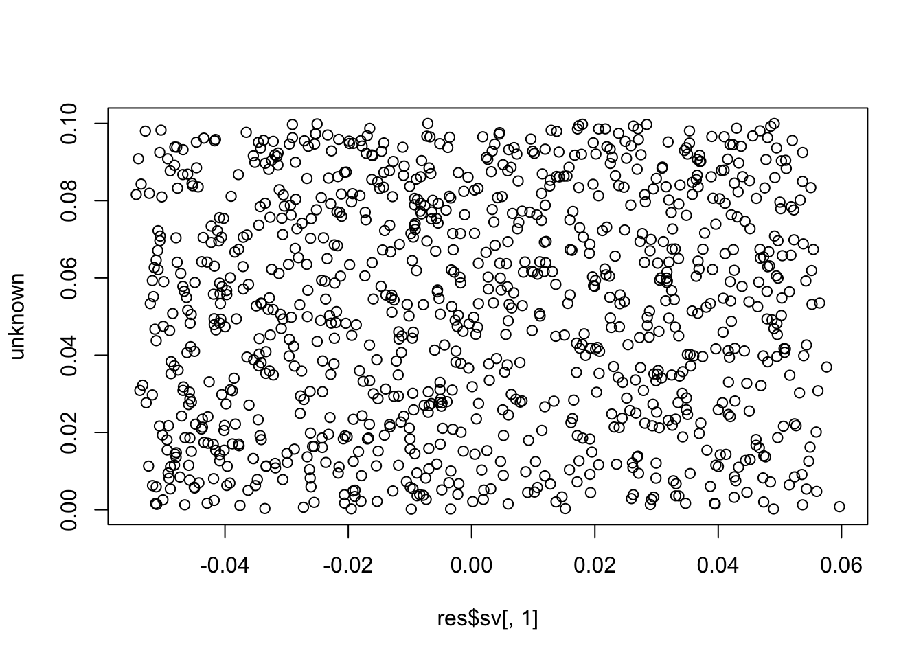


cor(res$sv[,1], unknown) # these SVs are not the unknown factor (correlation ~= 0) 
# [1] 0.05699341
cor(res$sv[,2], unknown) 
# [1] -0.1317231
cor(res$sv[,3], unknown) 
# [1] 0.06301151
cor(res$sv[,4], unknown) 
# [1] -0.08444932
cor(res$sv[,5], unknown) 
# [1] 0.1239618

cor(res$sv[,1], known) # ... but are instead the known factor (correlation ~= +/-1) 
# [1] -0.9988192
cor(res$sv[,2], known) 
# [1] 0.9971117
cor(res$sv[,3], known) 
# [1] -0.9558875
cor(res$sv[,4], known) 
# [1] 0.9982102
cor(res$sv[,5], known) 
# [1] -0.9934994

Compare to just naively taking the first PC of the residual matrix.

library(limma) 
# 
# Attaching package: 'limma'
# The following object is masked from 'package:BiocGenerics':
# 
#     plotMA
resid <- removeBatchEffect(log(assay(se)+1), covariates=known) 
pr.out <- prcomp(t(resid), rank.=1) 
plot(pr.out$x[,1], unknown)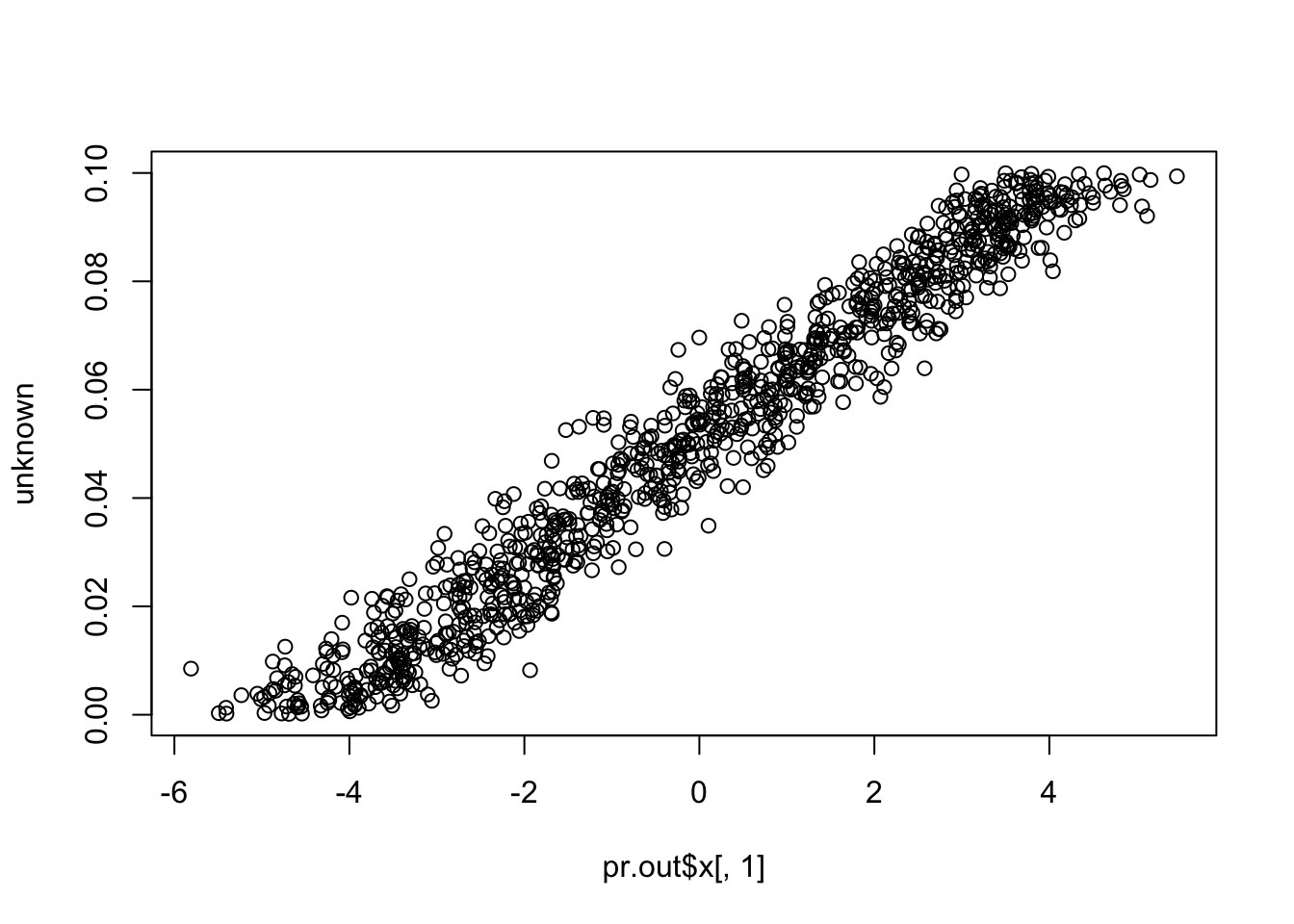

cor(pr.out$x[,1], unknown) # close to (-)1 
# [1] 0.9766822
cor(pr.out$x[,1], known) # close to zero. 
# [1] 2.35573e-17

Compare to SVA

library(sva)
mod1 <- model.matrix(~known)
mod0 <- cbind(mod1[,1])
sva.res = svaseq(counts,mod1,mod0, n.sv=5)$sv
# Number of significant surrogate variables is:  5 
# Iteration (out of 5 ):1  2  3  4  5
plot(sva.res[,1], unknown)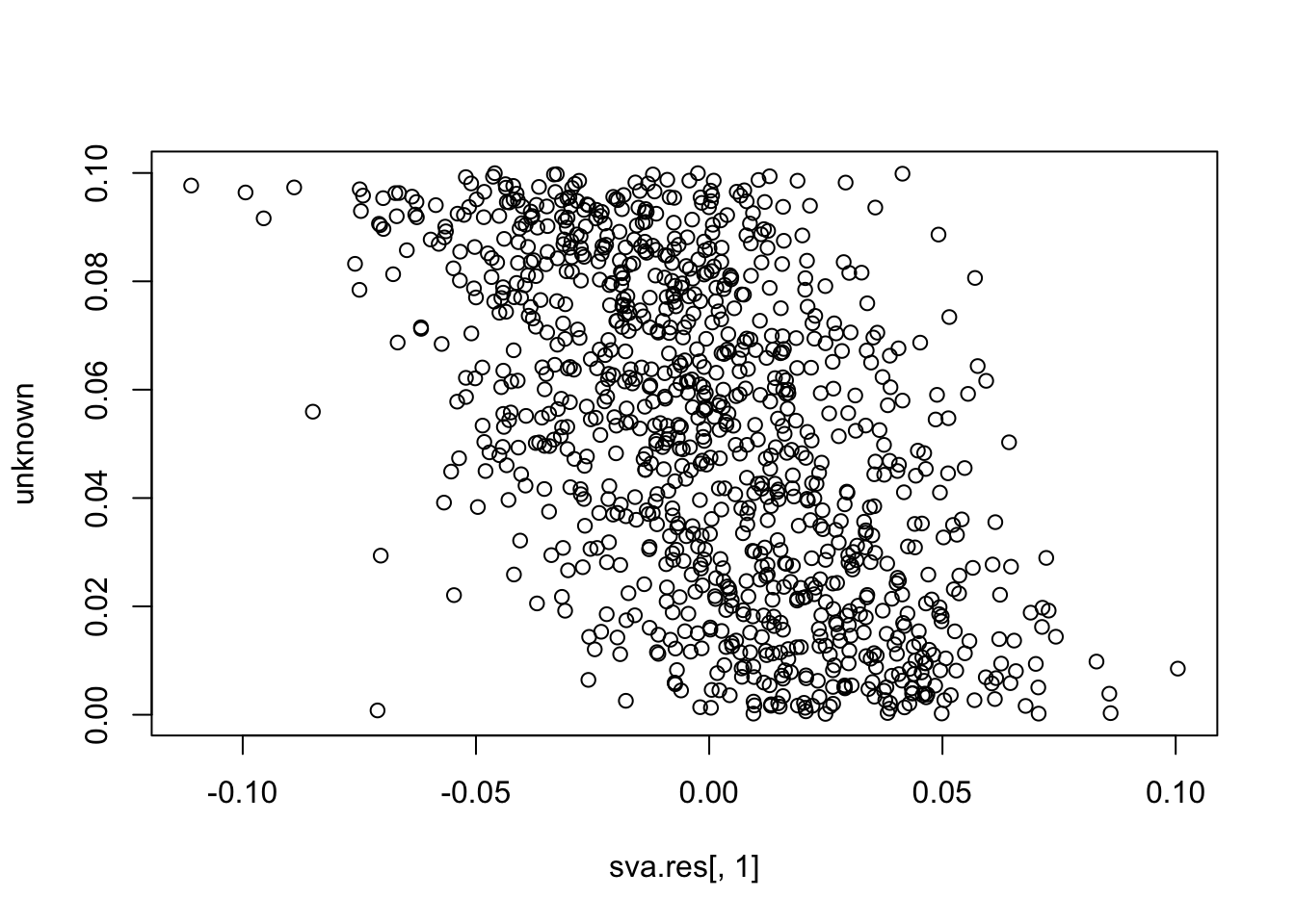

plot(sva.res[,1], known)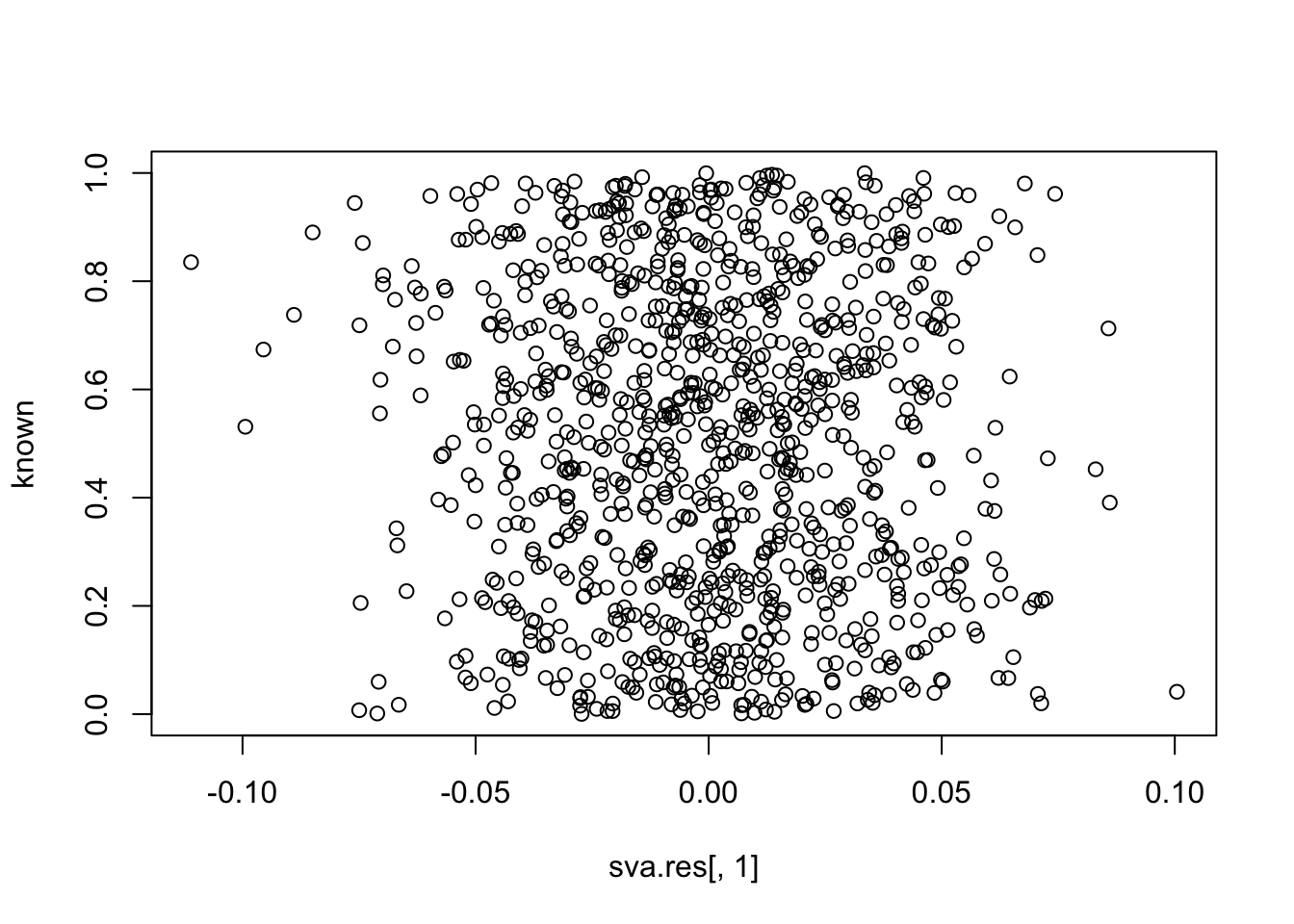

cor(sva.res[,1], unknown) # -0.55
# [1] -0.5522043
cor(sva.res[,1], known) # close to zero. 
# [1] -0.04603016

Simulation 2

set.seed(10000) 
known <- runif(1000) 
unknown <- runif(1000) 

ngenes <- 5000 
known.effect <- rnorm(ngenes, sd=2) 
unknown.effect <- rnorm(ngenes, sd=2) 
mat <- outer(known.effect, known) + 
outer(unknown.effect, unknown) + 
2 # to get decent-sized counts 

counts <- matrix(rpois(length(mat), lambda=2^mat), nrow=ngenes) 
library(SummarizedExperiment) 
se <- SummarizedExperiment(list(counts=counts)) 

library(iasva) 
design <- model.matrix(~known) 
res <- iasva(se, design, num.sv=5, permute = FALSE) 
# IA-SVA running...
# 
# SV 1 Detected!
# 
# SV 2 Detected!
# 
# SV 3 Detected!
# 
# SV 4 Detected!
# 
# SV 5 Detected!
# 
# # of significant surrogate variables: 5

cor(res$sv[,1], unknown) # first SV is the unknown factor. 
# [1] -0.9960557
cor(res$sv[,2], unknown) 
# [1] 0.7637275
cor(res$sv[,3], unknown) 
# [1] 0.7564822
cor(res$sv[,4], unknown) 
# [1] -0.7629373
cor(res$sv[,5], unknown) 
# [1] 0.4760279

cor(res$sv[,1], known) 
# [1] -0.004959888
cor(res$sv[,2], known) # but SVs 2-5 are correlated with the known factor... 
# [1] -0.7014209
cor(res$sv[,3], known) 
# [1] -0.7076734
cor(res$sv[,4], known) 
# [1] -0.476617
cor(res$sv[,5], known) 
# [1] -0.8898334


# Compare to SVA
library(sva)
mod1 <- model.matrix(~known)
mod0 <- cbind(mod1[,1])
sva.res = svaseq(counts,mod1,mod0, n.sv=3)$sv
# Number of significant surrogate variables is:  3 
# Iteration (out of 5 ):1  2  3  4  5
plot(sva.res[,1], unknown)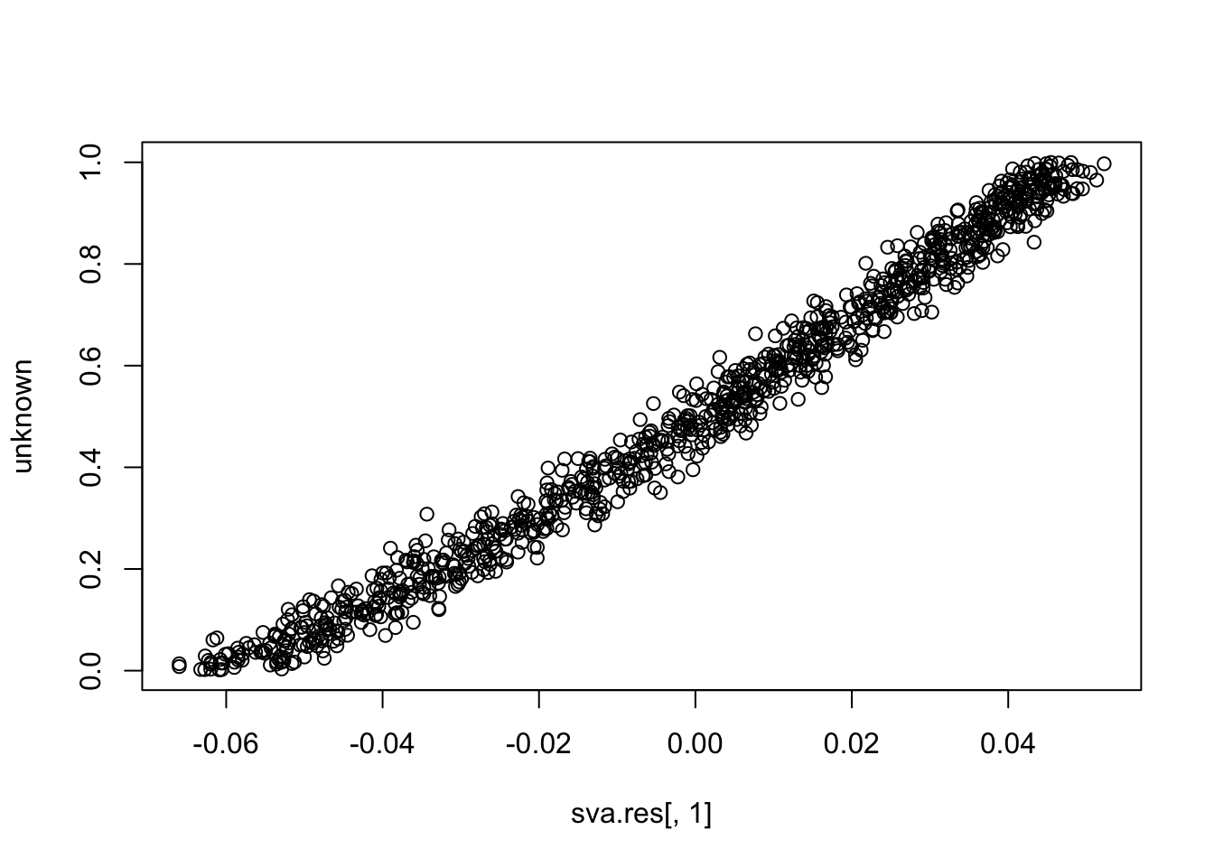

plot(sva.res[,1], known)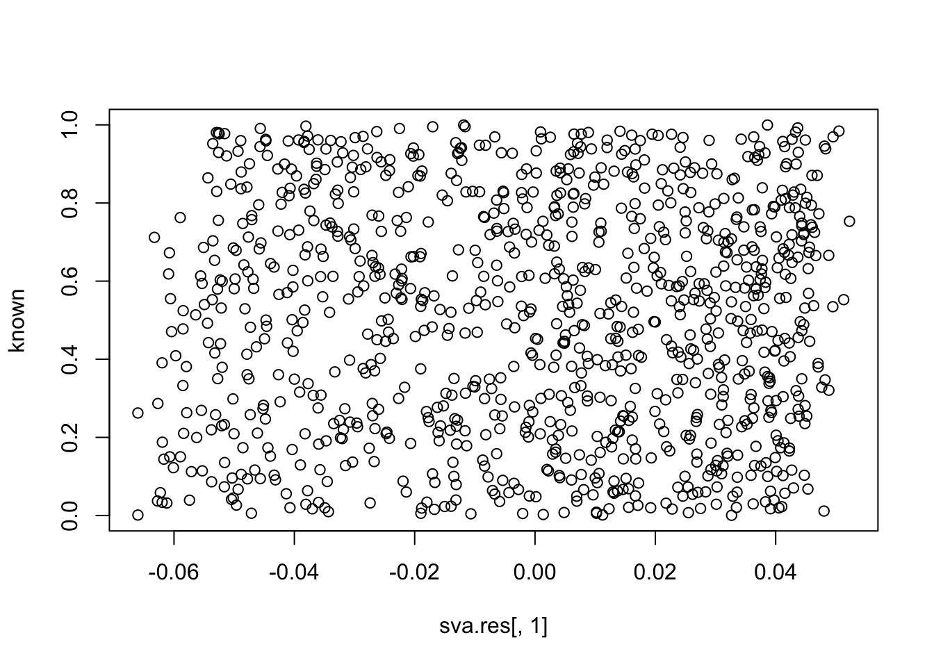

cor(sva.res[,1], unknown) # close to (-)1 
# [1] 0.989786
cor(sva.res[,2], unknown)
# [1] 0.03346006
cor(sva.res[,3], unknown) 
# [1] -0.01770404

cor(sva.res[,1], known) # close to zero. 
# [1] 0.0007217181
cor(sva.res[,2], known)
# [1] -0.04076436
cor(sva.res[,3], known)
# [1] -0.04114449

Corrected Simulation 1 with low correlation btw known and hidden factors

# Setting up the known and unknown factors. 
set.seed(10000) 
sample.size <- 100
ngenes <- 5000
# CORRECTEION: Here, we simulate factors with two levels (0 or 1).
factor.prop <- 0.5
flip.prob <- 0.5 ## to make no correlation btw known and hidden factors
known <- c(rep(-1,each=sample.size*factor.prop),rep(1,each=sample.size-(sample.size*factor.prop)))
coinflip = rbinom(sample.size,size=1,prob=flip.prob)
unknown = known*coinflip + -known*(1-coinflip)
cor(known, unknown)
# [1] -0.06030227

# Generating Poisson count data from log-normal means. 
ngenes <- 5000 
known.effect <- rnorm(ngenes, sd=2) 
unknown.effect <- rnorm(ngenes, sd=2) ## CORRECTION: to make factor with weach effect size, we use 1 as SD here.

mat <- outer(known.effect, known) + outer(unknown.effect, unknown) + 2 # to get decent-sized counts 

counts <- matrix(rpois(length(mat), lambda=2^mat), nrow=ngenes)
se <- SummarizedExperiment(assays=counts) 

# Running IA-SVA, version 0.99.3. 
library(iasva) 
design <- model.matrix(~known) 
## CORRECTION: IASVA doesn't accept the constant term of design matrix, so we use design[,-1] instead of design
res <- iasva(se, as.matrix(design[,-1]), num.sv=5, permute=FALSE) #num.p=20, threads=8) 
# IA-SVA running...
# 
# SV 1 Detected!
# 
# SV 2 Detected!
# 
# SV 3 Detected!
# 
# SV 4 Detected!
# 
# SV 5 Detected!
# 
# # of significant surrogate variables: 5
plot(res$sv[,1], unknown)


cor(res$sv[,1], unknown) # these SVs are not the unknown factor (correlation ~= 0) 
# [1] -0.9978671
cor(res$sv[,2], unknown) 
# [1] -0.8506371
cor(res$sv[,3], unknown) 
# [1] -0.9022145
cor(res$sv[,4], unknown) 
# [1] -0.8897027
cor(res$sv[,5], unknown) 
# [1] 0.7309927

cor(res$sv[,1], known) # ... but are instead the known factor (correlation ~= +/-1) 
# [1] 0.1251865
cor(res$sv[,2], known) 
# [1] 0.5759605
cor(res$sv[,3], known) 
# [1] 0.4847508
cor(res$sv[,4], known) 
# [1] 0.5043688
cor(res$sv[,5], known) 
# [1] -0.7206372

# Compare to just naively taking the first PC of the residual matrix. 
library(limma) 
resid <- removeBatchEffect(log(assay(se)+1), covariates=known) 
pr.out <- prcomp(t(resid), rank.=1) 
plot(pr.out$x[,1], unknown)

cor(pr.out$x[,1], unknown) # close to (-)1 
# [1] -0.9981718
cor(pr.out$x[,1], known) # close to zero. 
# [1] -7.096324e-18


# Compare to SVA
library(sva)
mod1 <- model.matrix(~known)
mod0 <- cbind(mod1[,1])
sva.res = svaseq(counts,mod1,mod0, n.sv=3)$sv
# Number of significant surrogate variables is:  3 
# Iteration (out of 5 ):1  2  3  4  5
plot(sva.res[,1], unknown)

plot(sva.res[,1], known)

cor(sva.res[,1], unknown) # close to (-)1 
# [1] 0.9976468
cor(sva.res[,1], known) # close to zero. 
# [1] 0.005334052

Corrected Simulation 1 with high correlation btw known and hidden factors

# Setting up the known and unknown factors. 
set.seed(10000) 
sample.size <- 100 ##CORRECTION, to reduce the computational burden, we used smaller sample size.
ngenes <- 5000
# CORRECTEION: Here, we simulate factors with two levels (0 or 1).
factor.prop <- 0.5
flip.prob <- 0.8 ## to make no correlation btw known and hidden factors
known <- c(rep(-1,each=sample.size*factor.prop),rep(1,each=sample.size-(sample.size*factor.prop)))
coinflip = rbinom(sample.size,size=1,prob=flip.prob)
unknown = known*coinflip + -known*(1-coinflip)
cor(known, unknown)
# [1] 0.6940221

# Generating Poisson count data from log-normal means. 
ngenes <- 5000 
known.effect <- rnorm(ngenes, sd=2) 
unknown.effect <- rnorm(ngenes, sd=2) ## CORRECTION: to make factor with weach effect size, we use 1 as SD here.

mat <- outer(known.effect, known) + outer(unknown.effect, unknown) + 2 # to get decent-sized counts 

counts <- matrix(rpois(length(mat), lambda=2^mat), nrow=ngenes)
se <- SummarizedExperiment(assays=counts) 

# Running IA-SVA, version 0.99.3. 
library(iasva) 
design <- model.matrix(~known) 
## CORRECTION: IASVA doesn't accept the constant term of design matrix, so we use design[,-1] instead of design
res <- iasva(se, as.matrix(design[,-1]), num.sv=5, permute=FALSE) #num.p=20, threads=8) 
# IA-SVA running...
# 
# SV 1 Detected!
# 
# SV 2 Detected!
# 
# SV 3 Detected!
# 
# SV 4 Detected!
# 
# SV 5 Detected!
# 
# # of significant surrogate variables: 5

plot(res$sv[,1], unknown)

cor(res$sv[,1], unknown) # accurately estimate the hidden factor (correlation ~= +/-1) 
# [1] 0.9787781
cor(res$sv[,2], unknown) 
# [1] 0.9238274
cor(res$sv[,3], unknown) 
# [1] 0.9272298
cor(res$sv[,4], unknown) 
# [1] 0.9283517
cor(res$sv[,5], unknown) 
# [1] -0.8907946

cor(res$sv[,1], known) # ... but are instead the known factor (correlation ~= +/-1) 
# [1] 0.8263641
cor(res$sv[,2], known) 
# [1] 0.9164418
cor(res$sv[,3], known) 
# [1] 0.91305
cor(res$sv[,4], known) 
# [1] 0.9116705
cor(res$sv[,5], known) 
# [1] -0.9448956

res1 <- iasva(se, as.matrix(design[,-1]), threads=8) 
# IA-SVA running...
# 
# SV 1 Detected!
# 
# SV 2 Detected!
# 
# # of significant surrogate variables: 2
plot(res1$sv[,1], unknown)

cor(res1$sv[,1], unknown) # accurately estimate the hidden factor (correlation ~= +/-1) 
# [1] 0.9787781
cor(res1$sv[,2], unknown) # 
# [1] -0.9238274

# Compare to just naively taking the first PC of the residual matrix. 
library(limma) 
resid <- removeBatchEffect(log(assay(se)+1), covariates=known) 
pr.out <- prcomp(t(resid), rank.=1) 
plot(pr.out$x[,1], unknown)

cor(pr.out$x[,1], unknown) # close to (-)1 
# [1] 0.719475
cor(pr.out$x[,1], known) # close to zero. 
# [1] 3.376059e-16


# Compare to SVA
library(sva)
mod1 <- model.matrix(~known)
mod0 <- cbind(mod1[,1])
sva.res = svaseq(counts,mod1,mod0, n.sv=3)$sv
# Number of significant surrogate variables is:  3 
# Iteration (out of 5 ):1  2  3  4  5
plot(sva.res[,1], unknown)

plot(sva.res[,1], known)

cor(sva.res[,1], unknown) # close to (-)1 
# [1] 0.7275183
cor(sva.res[,1], known) # close to zero. 
# [1] 0.01369329

Session information

sessionInfo()
# R version 3.5.0 (2018-04-23)
# Platform: x86_64-apple-darwin15.6.0 (64-bit)
# Running under: macOS Sierra 10.12.6
# 
# Matrix products: default
# BLAS: /Library/Frameworks/R.framework/Versions/3.5/Resources/lib/libRblas.0.dylib
# LAPACK: /Library/Frameworks/R.framework/Versions/3.5/Resources/lib/libRlapack.dylib
# 
# locale:
# [1] en_US.UTF-8/en_US.UTF-8/en_US.UTF-8/C/en_US.UTF-8/en_US.UTF-8
# 
# attached base packages:
# [1] parallel  stats4    stats     graphics  grDevices utils     datasets 
# [8] methods   base     
# 
# other attached packages:
#  [1] limma_3.36.2                SummarizedExperiment_1.10.1
#  [3] DelayedArray_0.6.1          matrixStats_0.53.1         
#  [5] Biobase_2.40.0              GenomicRanges_1.32.3       
#  [7] GenomeInfoDb_1.16.0         IRanges_2.14.10            
#  [9] S4Vectors_0.18.3            BiocGenerics_0.26.0        
# [11] sva_3.28.0                  BiocParallel_1.14.2        
# [13] genefilter_1.62.0           mgcv_1.8-23                
# [15] nlme_3.1-137                iasva_0.99.3               
# 
# loaded via a namespace (and not attached):
#  [1] Rcpp_0.12.17           compiler_3.5.0         git2r_0.21.0          
#  [4] workflowr_1.0.1        XVector_0.20.0         R.methodsS3_1.7.1     
#  [7] R.utils_2.6.0          bitops_1.0-6           tools_3.5.0           
# [10] zlibbioc_1.26.0        bit_1.1-14             digest_0.6.15         
# [13] memoise_1.1.0          RSQLite_2.1.1          annotate_1.58.0       
# [16] evaluate_0.10.1        lattice_0.20-35        Matrix_1.2-14         
# [19] DBI_1.0.0              yaml_2.1.19            GenomeInfoDbData_1.1.0
# [22] stringr_1.3.1          knitr_1.20             cluster_2.0.7-1       
# [25] bit64_0.9-7            rprojroot_1.3-2        grid_3.5.0            
# [28] AnnotationDbi_1.42.1   survival_2.42-3        XML_3.98-1.11         
# [31] rmarkdown_1.9          irlba_2.3.2            blob_1.1.1            
# [34] magrittr_1.5           whisker_0.3-2          splines_3.5.0         
# [37] backports_1.1.2        htmltools_0.3.6        xtable_1.8-2          
# [40] stringi_1.2.2          RCurl_1.95-4.10        R.oo_1.22.0

This reproducible R Markdown analysis was created with workflowr 1.0.1

Reviewer 2 Simulation

Donghyung Lee

2018-07-31

Simulation 1

Compare to just naively taking the first PC of the residual matrix.

Compare to SVA

Simulation 2

Corrected Simulation 1 with low correlation btw known and hidden factors

Corrected Simulation 1 with high correlation btw known and hidden factors

Session information