Computational Graphs - Symbolic Computation
Christoph Heindl 2017, https://github.com/cheind/py-cgraph/
This is part two in a series about computational graphs and their applications. The first part covered theoretical foundations of computational graphs and algorithms to perform forward function evaluation and backward derivative computations.
This part will focus on developing Python code that allows numeric and symbolic differentiation of arbitrary (real valued) functions.
CGraph
CGraph is the name of the Python library to be developed during the remainder of this notebook. While the code inside the notebook is functional, a separate, self-contained and enhanced implementation of CGraph is available cgraph.py. The most striking difference is that the provided code supports more built-in functions and supports evaluating multiple parameter sets at once making it more performant than the notebook version.
CGraph performs numeric and symbolic differentiation using backpropagation. The code below shows a sample session.
import cgraph as cg

x = cg.Symbol('x')
y = cg.Symbol('y')
z = cg.Symbol('z')

f = (x * y + 3) / (z - 2)

# Evaluate function
cg.value(f, {x:2, y:3, z:3}) # 9.0

# Partial derivatives (numerically)
d = cg.numeric_gradient(f, {x:2, y:3, z:3})
d[x] # df/dx 3.0
d[z] # df/dz -9.0

# Partial derivatives (symbolically)
d = cg.symbolic_gradient(f)
cg.simplify(d[x]) # (y*(1/(z - 2)))
cg.value(d[x], {x:2, y:3, z:3}) # 3.0

# Higher order derivatives
ddx = cg.symbolic_gradient(d[x])
cg.simplify(ddx[y]) # ddf/dxdy
# (1/(z - 2))
Python 3.5 will be used for development. The reader is assumed to be familiar with its concepts including generators and decorators. Also a technique called monkey patching will be used to iteratively refine classes introduced previously.
Expression trees
Before diving into code, we need to cover the concept of expression trees. Expression trees will be used to represent function decompositions. While they are not a fundamentally new concept they deserve some words at this point.
An expression tree is similar to the computational graphs introduced, but the arrows by default point backwards. It turns out that representing functions in a tree like manner (top node is the function itself, function parameters are leafs) simplifies development dramatically compared to CGs.
Take the CG of the toy example used $f(x,y)=(x+y)x$
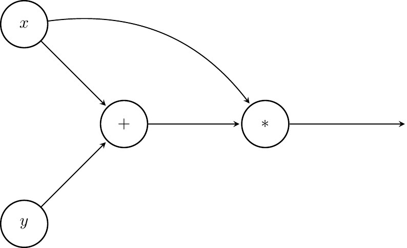
The following expression tree represents the same function
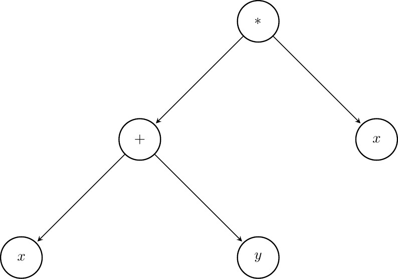
Notice that we now have a tree like structure. Our root node is the final operation to be executed to receive the result of $f(x,y)$. $x$ shows up twice now. Finding the value of an expression tree requires to compute values of nodes in lower layers first and bubble information up towards the root node. Backpropagation on the other hand can start at the root and then follow the forward edges. When computing derivatives not much changes: we will have a summation over all paths from the top that lead to a given node and every node will perform the product of two terms (chain rule) that is send to its children.
Representing expression trees
First we need to come up with a way to represent expression trees. In CGraph we will have a base class Node that manages child references. Derived classes will actually implement operations, symbols and constants.
class Node:
    """A base class for operations, symbols and constants in an expression tree."""

    def __init__(self, nary=0):
        self.children = [None]*nary

    def __repr__(self):
        return self.__str__()
Node just tracks references to its children. Operations can be binary (e.g. addition), unary (e.g cosine) or don't have children at all (e.g. symbols). We can also think of n-ary functions such as summation.
Next, we'll define the leaf nodes Symbol and Constant
class Symbol(Node):
    """Represents a terminal node that might be associated with a scalar value."""

    def __init__(self, name):
        super(Symbol, self).__init__(nary=0)
        self.name = name

    def __str__(self):
        return self.name

    def __hash__(self):
        return hash(self.name)

    def __eq__(self, other):
        if isinstance(other, self.__class__):
            return self.name == other.name
        else:
            return False
Symbols are uniquely identified by their name, like $x$. They don't have any children. When printed we print the name of the symbol.
class Constant(Node):
    """Represents a constant value in an expression tree."""

    def __init__(self, value):
        super(Constant, self).__init__(nary=0)
        self.value = value

    def __str__(self):
        return str(self.value)
Constants are just 'immutable' values.
Next we start to add operations. Here we will just work with addition and multiplication. cgraph.py contains more operations. Once you know how to implement them it will be easy to add new ones.
class Add(Node):
    """Binary addition of two nodes."""

    def __init__(self):
        super(Add, self).__init__(nary=2)

    def __str__(self):
        return '({}+{})'.format(str(self.children[0]), str(self.children[1]))

class Mul(Node):
    """Binary multiplication of two nodes."""

    def __init__(self):
        super(Mul, self).__init__(nary=2)

    def __str__(self):
        return '({}*{})'.format(str(self.children[0]), str(self.children[1]))
Add and Mul don't do much yet expect that stating that they are binary functions plus some pretty printing (recursively calling __str__ on its children).
What follows is a helper function that builds the expression tree for our toy function $f(x,y)=(x+y)x$. This looks a bit clumsy right now but we'll improve the syntax as we go.
def gen_f(x, y):
    a = Add()
    a.children[0] = x
    a.children[1] = y

    m = Mul()
    m.children[0] = a
    m.children[1] = x

    return m

x = Symbol('x')
y = Symbol('y')
f = gen_f(x, y)
f
Computing function values
As mentioned earlier, to compute the value of an expression tree we need to bubble up information from layers further down in hierarchy up to the root. Traversing expression trees can be performed in multiple ways. What we are looking for is depth-first-search in post-order. There are many ways to implement the traversal, i've chosen the recursive generator approach because of its shortness.
def postorder(node):
    """ Yields all nodes discovered by depth-first-search in post-order."""
    for c in node.children:
        yield from postorder(c)
    yield node
[n for n in postorder(f)]
As expected children are evaluated before their parental nodes.
Next, define a method that computes the value of the expression tree.
def values(f, fargs):
    """Returns a dictionary of computed values for each node in the expression tree including `f`."""
    v = {}
    v.update(fargs)
    for n in postorder(f):
        if not n in v:
            v[n] = n.compute_value(v)
    return v
This method calls compute_value(values) for each node and expects the node to return its value. Since we haven't defined this function for our nodes yet, it's time to do so. Also note that fargs will be assumed to contain the values for the symbols in the expression tree.
# Monkey patching for compute_value

Symbol.compute_value = lambda self, values: values[self]
Constant.compute_value = lambda self, values : self.value
Add.compute_value = lambda self, values: values[self.children[0]] + values[self.children[1]]
Mul.compute_value = lambda self, values: values[self.children[0]] * values[self.children[1]]
After monkey patching for compute_value we can evaluate f by
values(f, {x:2, y:3})
values computes the values for all nodes in the expression tree. However, most often we will be interested in the value of f only. Here's a handy shortcut named value to do so.
def value(f, fargs):
    """Shortcut for `values(f, fargs)[f]`."""
    return values(f, fargs)[f]

value(f, {x:2, y:3})
Syntactic sugar
Before continuing, it makes sense to define Python's internal methods for 'overloading' the + and * operation of Nodes. First, we'll define a decorator that will wrap plain numbers to Constants.
from numbers import Number

def wrap_args(func):
    """Wraps function arguments that are numbers as Constant objects."""
    def wrapped(*args, **kwargs):
        new_args = []
        for a in args:
            if isinstance(a, Number):
                a = Constant(a)
            new_args.append(a)
        return func(*new_args, **kwargs)
    return wrapped
Next, we'll define some free functions that perform assembling addition and multiplication nodes from arguments. By convention these free functions will start with the prefix sym_ (for symbolic). When adding new functionality you should always provide such a function (e.g sym_pow, sym_cos).
@wrap_args
def sym_add(x, y):
    """Returns a new node that represents of `x+y`."""
    n = Add()
    n.children[0] = x
    n.children[1] = y
    return n

@wrap_args
def sym_mul(x, y):
    """Returns a new node that represents of `x*y`."""
    n = Mul()
    n.children[0] = x
    n.children[1] = y
    return n
Finally we monkey patch Node to support + and * operations
Node.__add__ = lambda self, other: sym_add(self, other)
Node.__radd__ = lambda self, other: sym_add(other, self)
Node.__mul__ = lambda self, other: sym_mul(self, other)
Node.__rmul__ = lambda self, other: sym_mul(other, self)
Note that the __r* methods are also provided so that expressions of the type n*3 and 3*n work equally well. With that in place we can rewrite gen_f introduced by simply stating
f = (x + y)*x
f
Computing numeric derivatives
Next we will turn our attention to the backpropagation for computing numerical derivatives. First another traversal will be needed. One that visits all nodes on the same level before moving on to the next level. Such a traversal is called breadth-first-search and it can also be implemented in numerous ways.
The way it is implemented here is based on a generator that uses a queue internally. Additionally, when performing backpropagation, we'd like to communicate values back to the generator for the children of the current node. We then expect the handed values to be passed to us when we visit the corresponding child.
Doing so turns the generator into co-routine.
def bfs(node, node_data):
    """Yields all nodes and associated data in breadth-first-search."""
    q = [(node, node_data)]
    while q:
        t = q.pop(0)
        node_data = yield t
        for idx, c in enumerate(t[0].children):
            q.append((c, node_data[idx]))
Next, numeric_gradient is introduced. It takes an expression tree and function arguments for the contained symbols. It returns all numeric partial derivatives with respect to the root node passed.
from collections import defaultdict

def numeric_gradient(f, fargs):
    """Computes the numerical partial derivatives of `f` with respect to all nodes."""
    vals = values(f, fargs)
    derivatives = defaultdict(int) # by default 0 is the derivative for unknown nodes.

    gen = bfs(f, 1)
    try:
        n, in_grad = next(gen)
        while True:
            derivatives[n] += in_grad
            local_grad = n.compute_gradient(vals)
            n, in_grad = gen.send([l*in_grad for l in local_grad])
    except StopIteration:
        return derivatives
First, numeric_gradient performs a forward pass to compute all function values. Next, breadth-first-search is kicked of by f and a value of 1. Then for each node visited, we accumulate incoming partial derivatives send along from previous computations. Next, the 'isolated' gradient is computed. We communicate back the local gradient times incoming partial derivative as explained in the backpropagation introduction before. Once we've hit the last node, a dictionary of partial derivatives is returned.
numeric_gradient tries to call compute_gradient(values) for every node. compute_gradient is expected to take in a values dictionary and return the isolated partial derivative for each child in array form. As always, lets monkey patch.
# Monkey patch for compute_gradient
Symbol.compute_gradient = lambda self, values: [] # Nothing todo
Constant.compute_gradient = lambda self, values: [] # Nothing todo

Add.compute_gradient = lambda self, values: [1, 1] # dx+y/dx = 1, dx+y/dy = 1
Mul.compute_gradient = lambda self, values: [values[self.children[1]], values[self.children[0]]] # dx*y/dx = y, dx*y/dy = x
The isolated gradients for Add and Mul should look familiar to you. If not, you should go back to the introduction on computational graphs in the first part of this series. With that in place we can now compute numeric derivatives.
numeric_gradient(f, {x:2, y:3})
$\frac{\mathrm{d}f(x,y)}{\mathrm{d}x}\Bigr|_{\substack{x=2\\y=3}} = 7$ and $\frac{\mathrm{d}f(x,y)}{\mathrm{d}y}\Bigr|_{\substack{x=2\\y=3}} = 2$ is what we expect.
Additionally, the result also contains derivatives for intermediate nodes. Here are some more examples.
numeric_gradient(x*x+y*y, {x:2, y:3})
z = Symbol('z')
numeric_gradient((x+3)*(y+4)*z*z, {x:2, y:3, z:5})
Computing symbolic derivatives
Now that we can compute numeric derivatives, one might wonder if we could do the same symbolically, i.e instead of returning a number we return some expression tree. Clearly such a feature would be beneficial as it would allow computation of higher order derivatives. Additionally, pre-factoring the derivative expressions might be favorable when invoking the derivative evaluation multiple times.
Turns out modifying the numeric gradient computation for symbolic computation is straight forward. All that needs to be done is to return appropriate Nodes instead of numeric values. Infact with the overloaded + and * operations in place for nodes, the symbolic gradient computation looks nearly identical to numeric_gradient defined earlier.
Here it is, symbolic_gradient
def symbolic_gradient(f):
    """Computes the symbolic partial derivatives of `f` with respect to all nodes."""
    derivatives = defaultdict(lambda: Constant(0))

    gen = bfs(f, Constant(1))
    try:
        n, in_grad = next(gen) # Need to use edge info when expressions are reused!
        while True:
            derivatives[n] = derivatives[n] + in_grad
            local_grad = n.symbolic_gradient()
            n, in_grad = gen.send([l * in_grad for l in local_grad])
    except StopIteration:
        return derivatives
We use Constant instead of plain numbers and a invoke symbolic_gradient. The operations + and * seen above refer to the binary operation defined between Node objects.
As always, let's monkey patch for symbolic_gradient.
# Monkey patch for symbolic_gradient
Symbol.symbolic_gradient = lambda self: [] # Nothing todo
Constant.symbolic_gradient = lambda self: [] # Nothing todo

Add.symbolic_gradient = lambda self: [Constant(1), Constant(1)] # dx+y/dx = 1, dx+y/dy = 1
Mul.symbolic_gradient = lambda self: [self.children[1], self.children[0]] # dx*y/dx = y, dx*y/dy = x
Let's test.
symbolic_gradient(f)
Have a look at $x$. It claims derivative of $f$ with respect to $x$ is equal to ((0 + ((x + y)*1)) + (1*(x*1))). After massaging the terms you indeed find that this is the same as $2x+y$. Although not very readable, the reported results are correct. Readability will be covered in the next section.
Since the returned dictionary contains expressions made of Node objects, we can apply all functions developed so far onto them.
d = symbolic_gradient(f)
print('df/dx at (x=2,y=3) is {}'.format(value(d[x], {x:2, y:3})))
print('df/dy at (x=2,y=3) is {}'.format(value(d[y], {x:2, y:3})))

# Let's try second order derivatives
ddx = symbolic_gradient(d[x])
ddy = symbolic_gradient(d[y])
print('ddf/dxdx at (x=2,y=3) is {}'.format(value(ddx[x], {x:2, y:3})))
print('ddf/dxdy at (x=2,y=3) is {}'.format(value(ddx[y], {x:2, y:3})))
print('ddf/dydx at (x=2,y=3) is {}'.format(value(ddy[x], {x:2, y:3})))
print('ddf/dydy at (x=2,y=3) is {}'.format(value(ddy[y], {x:2, y:3})))
Adding new operations
Adding new operations to CGraph is not difficult. The following recipe sums up the necessary steps.
- Add a new class inheriting
Node - Add implementations for
compute_value,symbolic_gradientand forcompute_gradient - Provide one or more free function with prefix
sym_*that connects arguments as inputs for your operation. Use@wrap_argswhere appropriate. - Optionally provide
__str__ - Optionally add new
__*__methods inNodeto support improved syntax delegating tosym_*methods.
A word of caution: when computing numeric gradients through compute_gradient you might find yourself in a position of potentially dividing by zero or raising any other math expection. When this happens, gradient computation will stop. For example consider $f(x,y) = x^y$ and let $x=-1, y=2$. Then when evaluating the gradient for $y$ you will find that it corresponds to $x^y*log(x)$. Unfortunately $x$ is negative and so the value can not be computed. Python raises an exception and gradient computation fails. Now assume that you are not interested in the derivative with respect to $y$ at all, still you will get no result as gradient computation stopped after the exception.
CGraph handles this by using NANs instead of exceptions. Almost all operations that invoke NANs result in NAN, so they propagate nicely. CGraph uses numpy arrays as a basic container for values. Numpy by default turns these exceptions into NAN and issues a warning.
Expression simplification
Earlier we saw that symbolic differentiation produces hardly readable expressions, such as ((0+((x+y)∗1))+(1∗(x∗1))). In this section we will see how to simplify such expressions. Not only will this improve readability, but also give a better performance as lesser nodes need to be evaluated (pays off especially when you invoke it many times after simplification).
The way CGraph implements expression simplification is by traversing the computational graph while trying to apply simplification rules. Each rule acts on a single node and may produce a simplier version of that node. The new node 'replaces' the old node in an expression tree that is formed in parallel. That means that we won't fiddle around with the original expression tree given, but rather generate a expression tree that represents a simplified version of the original one.
First we will implement a rule filter decorator, a helper function and a single rule.
def applies_to(*klasses):
    """Decorates rule functions to match specific nodes in simplification."""

    def wrapper(func):
        def wrapped_func(node):
            if isinstance(node, klasses):
                return func(node)
            else:
                return node
        return wrapped_func
    return wrapper
Next, a helper function to check if a node is 'Constant' and has a specific value.
def is_const(node, value=None):
    """Returns true when the node is Constant and matched `value`."""
    if isinstance(node, Constant):
        if value is not None:
            return node.value == value
        else:
            return True
    return False
The first rule will be the rule for multiplication with the identity element $x*1=x$.
@applies_to(Mul)
def mul_identity_rule(node):
    """Simplifies `x*1` to `x`."""
    if is_const(node.children[0], 1):
        return node.children[1]
    elif is_const(node.children[1], 1):
        return node.children[0]
    else:
        return node
First notice that this rule will only applies to Mul nodes via the decorator. Next, if any of the children is a constant with value 1, it simply returns the other one.
Next comes simplify. It uses the post-order traversal introduced earlier and invokes rules for each node visited. In parallel it builds a new expression tree.
import copy

rules = [mul_identity_rule]
def simplify(node):
    """Returns a simplified version of the expression tree associated with `node`."""

    nodemap = {}
    for n in postorder(node):
        if isinstance(n, Symbol):
            continue

        nc = copy.copy(n)
        for i in range(len(nc.children)):
            c = nc.children[i]
            nc.children[i] = nodemap.get(c, c)
        for r in rules:
            nc = r(nc)
        nodemap[n] = nc

    return nodemap[node]
Applied to the expression from before
d = symbolic_gradient(f)
print(d[x]) # Hardly readable
print(simplify(d[x])) # A bit better
Quite an improvement. Here's one more rule simplifying $x+0=x$
@applies_to(Add)
def add_identity_rule(node):
    """Simplifies `x+0` to `x`."""
    if is_const(node.children[0], 0):
        return node.children[1]
    elif is_const(node.children[1], 0):
        return node.children[0]
    else:
        return node

rules.append(add_identity_rule)
print(simplify(d[x])) # Even better
You are not restricted to rules that operate on direct successors only. Any rule can look for a pattern in the entire subtree given by the input node. Here's one last rule that I would like to advertise: a rule that turns any subgraph that consists of Constants into a single constant.
k = x + x + x + x + x
d = symbolic_gradient(k)
print(d[x])
print(simplify(d[x]))
Here's the rule. What's special about it is that it uses value without passing any numeric values for symbols.
def eval_to_const_rule(node):
    """Simplifies every expression made of Constants only to a single Constant."""
    try:
        k = value(node, {})
        return Constant(k)
    except KeyError: # If node contains symbols we trap here
        return node

rules.append(eval_to_const_rule)

print(simplify(d[x]))
Summary
In this part CGraph a library for symbolic computation was introduced. CGraph is able to perform forward value propagation on expression trees and backward partial derivative computation in an efficient manner through the use of a scheme called backpropagation.