Computational Graphs
Christoph Heindl 2017, https://github.com/cheind/py-cgraph/
Computational graphs (CG) are a way of representing arbitrary mathematical function expression. A CG captures all expressions the function is made of, plus the necessary information on how information flows between expressions. Among other things, the study of CG leads to deeper understanding of calculus, especially computing derivatives. Given a function represented as a CG, one is able to compute partial derivatives by applying a single rule - the chain rule. CGs are well suited to be put into code, allowing us to automatically differentiate functions numerically or even symbolically.
CGs play an important rule in mathematical function optimization, especially when computing derivatives by hand becomes infeasable. Supervised training of neural networks, for example, maps to optimizing (minimizing) a cost function with respect to all the neural weights in the network chained in different layers. Optimization is usually performed using a gradient descent approach which requires first order derivatives of the cost function with respect to all the parameters in the network. As we will see, CGs not only make this doable but also provide an computationally efficient algorithm named backpropagation to compute the partial derivatives.
What this series will cover
This notebook and the following ones give an introduction into CGs and how to implement them in Python. By the end we will
- evaluate mathematical expressions represented as CGs,
- perform automatic differentiation to find numerically exact derivatives (up to floating point precision),
- perform symbolic differentiation to deduce higher order derivatives,
- simplify expressions to improve performance and readability.
What this series will not cover
To keep the code basis compact there are shortcomings to the developed framework. Foremost it is not complete. That means you won't be able to plugin every possible function and expect it return the correct result. This is mostly a problem of not providing derivatives for all the different elementary functions. However, the framework is structured in such a way that you will find it easy to add new blocks it and make it even more feature complete.
Also, we'll be mostly dealing with so called multivariate real-valued scalar functions $f:\mathbb {R} ^{n}\to \mathbb {R}$. In other words, we constrain our self to real values and functions that can have multiple inputs but will only output a single scalar value. A glimpse on how to use the framework for vector-valued functions will be given in a later part.
If you are looking for production ready libraries you might want to have a look at
In case you want to stick around and learn something about the fundamental concepts that drive these libraries, your are welcome.
Introduction to computational graphs (CG)
Consider a function
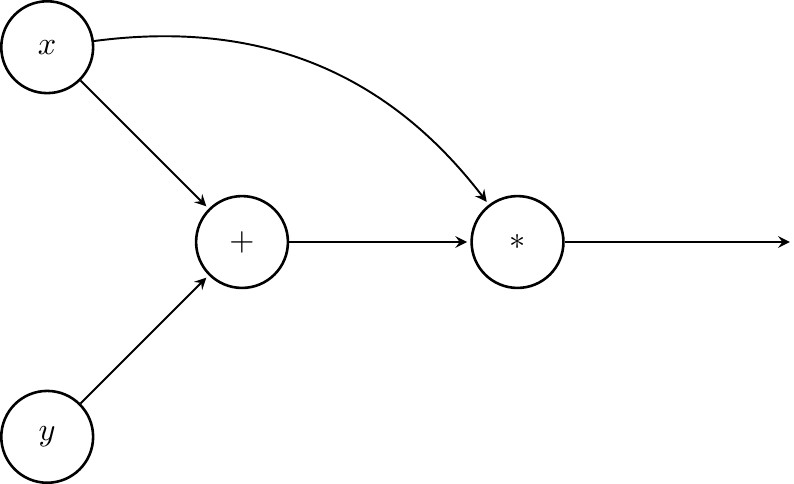
$$f(x,y) := (x + y)x$$We will call $x$ and $y$ symbols. $+$ and $*$ will be referred to as operations / functions or nodes. When we want to find the value of $f$, we first add up the values of $x$ and $y$ and then multiply the result by $x$. The value of the multiplication is what we call the value of $f(x,y)$. A CG represents such sequences of operations involving symbols using directed graphs. A graphical representation of CG for $f$ is shown below
Computing the value of $f(x,y)$
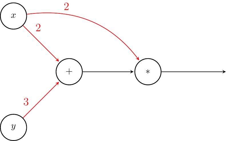
Computing the value of $f$ in the CG is a matter of following directed edges of the graph. Assume we want to evaluate $f(2,3)$. First, we send 2 and 3 along the out-edges of $x$ and $y$ respectively.
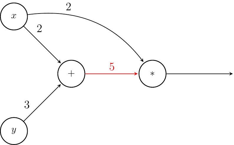
Next, we compute the value of $+$. Note that $*$ cannot be computed as one of its inputs, namely $+$ is missing.
Finally, we find value of $f$ by evaluating $*$
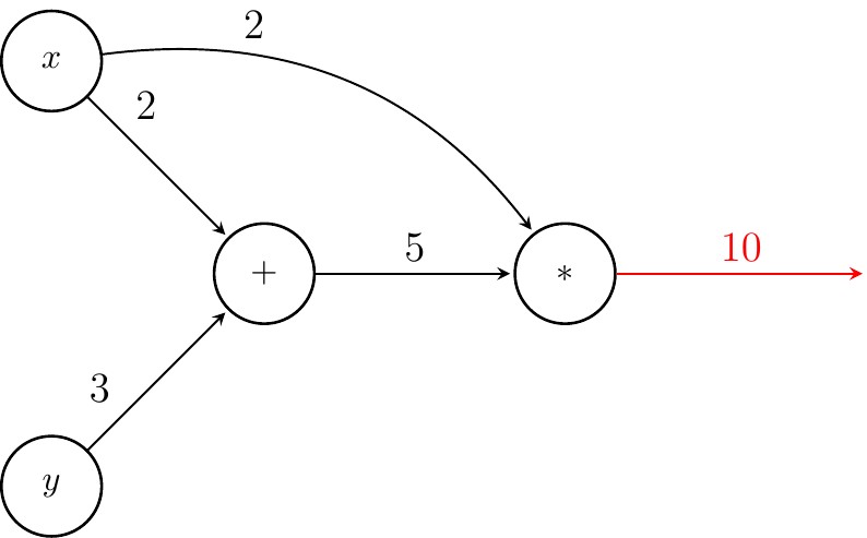
Finding the value of $f$ requires processing of all precessors of a node before evaluating the node itself. Such an ordering on a CG is called a topological order.
Computing the partial derivatives
We will now turn our attention towards computing partial derivatives. In order to do so, we will be a bit more abstract and use replace numbers by symbols for the outputs of all nodes. Like so.
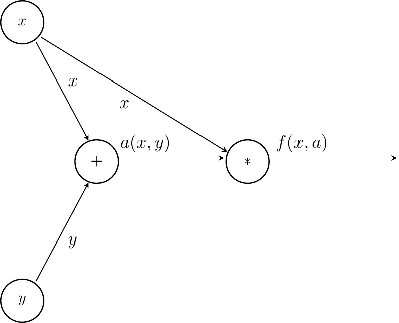
Please take a moment and convince yourself that $f(x,a) = f(x,y)$.
Partial derivatives of isolated nodes
Now consider any node in this CG in isolation, irrespectively of where it is located in the graph. When computing partial derivatives of isolated nodes with respect to their inputs, each input is treated as an abstract symbol. Therefore taking the derivative completely ignores the fact that each input might be the result a complex operation by itself. By taking this perspective of isolating nodes, computation of derivatives can be simplified.
For example, take the multiplication node $f(x,a) := ax$ in isolation. Computing the partial derivatives of $f(x,a)$ with respect to its inputs, requires
$$\frac{\mathrm{d}f(x,a)}{\mathrm{d}a}, \frac{\mathrm{d}f(x,a)}{\mathrm{d}x}$$to be found. This amounts to
$$\frac{\mathrm{d}f(x,a)}{\mathrm{d}a}=x, \frac{\mathrm{d}f(x,a)}{\mathrm{d}x}=a$$Similarily, for the addition node $a(x,y) := x+y$ we get
$$\frac{\mathrm{d}a(x,y)}{\mathrm{d}x}=1, \frac{\mathrm{d}a(x,y)}{\mathrm{d}y}=1$$In order to display the partial derivatives in the CG diagrams, we will use backward oriented arrows between nodes to which we attach the corresponding partial derivatives as shown below.
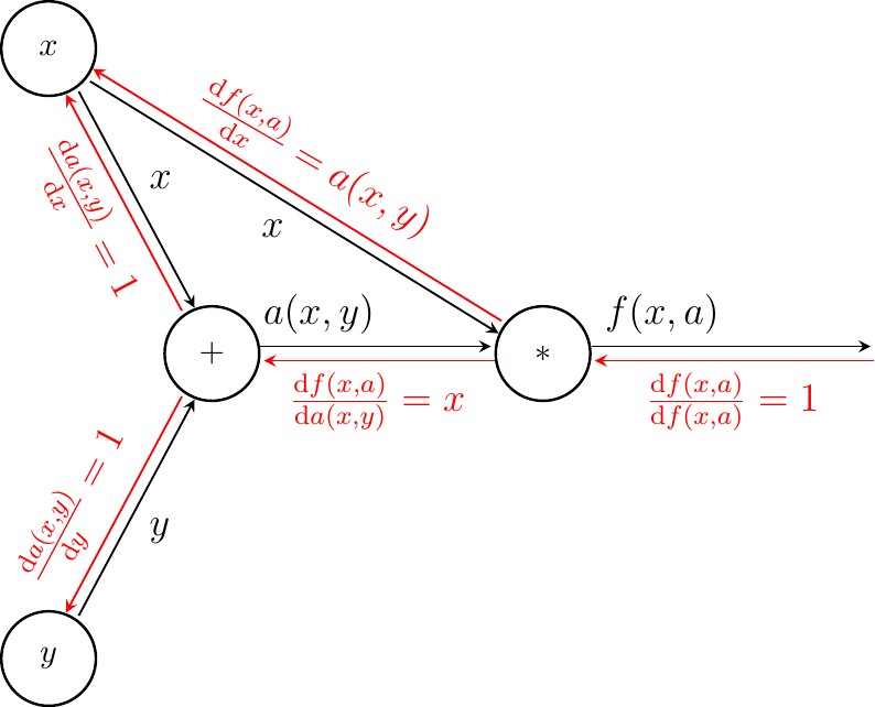
As shown, for each input arrow we generate a corresponding backward oriented arrow and assign it the partial derivative of the node's output with respect to the input. As a side node, when node has multiple inputs and a single output, and we stack all the partial derivatives in a vector, we call the result the gradient. For completness, when a node has multiple ouputs and inputs, we form a matrix for the resulting partial derivatives that we call the Jacobi Matrix.
Partial derivatives of nodes with respect to other nodes
To compute the partial derivative for any node $n$ with respect to the function $f(x,y):=(x+y)x$ in the CG diagram, one needs to
- Find all the backward paths starting from $f(x,a)$ reaching $n$.
- For each path build the product of partial derivatives along the chain of backward arrows.
- Sum over all path products of partial derivatives.
The above algorithm in pseudocode is known as the generalization of chain-rule. Take for example the partial derivative of $\frac{\mathrm{d}f(x,y)}{\mathrm{d}y}$ amounts to
$$\frac{\mathrm{d}f(x,y)}{\mathrm{d}y} = \frac{\mathrm{d}f(x,a)}{\mathrm{d}f(x,a)} \frac{\mathrm{d}f(x,a)}{\mathrm{d}a(x,y)} \frac{\mathrm{d}a(x,y)}{\mathrm{d}y} $$There is only one backward oriented path from $f(x,a)$ to $y$, so there is no explicit summation. Also note that $f(x,a)$ is equivalent to $f(x,y)$ by construction. By substitution (see CG diagram above) we find
$$\frac{\mathrm{d}f(x,y)}{\mathrm{d}y} = 1*x*1 = x$$Finding $\frac{\mathrm{d}f(x,y)}{\mathrm{d}x}$ is very similar, except that this time we have two paths in which $x$ can be reached from $f(x,a)$.
$$\frac{\mathrm{d}f(x,y)}{\mathrm{d}x} = \frac{\mathrm{d}f(x,a)}{\mathrm{d}f(x,a)} \frac{\mathrm{d}f(x,a)}{\mathrm{d}a(x,y)} \frac{\mathrm{d}a(x,y)}{\mathrm{d}x} + \frac{\mathrm{d}f(x,a)}{\mathrm{d}f(x,a)} \frac{\mathrm{d}f(x,a)}{\mathrm{d}x} $$By subsitution we get
$$\frac{\mathrm{d}f(x,y)}{\mathrm{d}x} = 1*x*1 + 1*a(x,y) = x + (x+y) = 2x+y$$Backward traversal of CGs using the chain-rule algorithm allows you to compute partial derivatives easily. Here is the general approach: first, decompose the function into operations simple enough, so you know how to compute isolated partial derivatives for individual nodes. Next, build a CG based on your decomposition. Apply the 3-step algorithm above to find partial derivatives of any two connected nodes in the CG (usually you do this for the input variables).
Backpropagation
While the algorithm introduced in previous section allows you to compute partial derivatives for any two nodes connected by a path in the CG, it is not efficient in doing so. Notice, the terms
$$\frac{\mathrm{d}f(x,a)}{\mathrm{d}f(x,a)}\frac{\mathrm{d}f(x,a)}{\mathrm{d}a(x,y)}$$appear in computations of both $\frac{\mathrm{d}f(x,y)}{\mathrm{d}x}$ and $\frac{\mathrm{d}f(x,y)}{\mathrm{d}y}$. While for our toy example CG the computational overhead is insignificant, but in a much larger CG (like neural networks) the number of shared terms might grow quickly and so does computation time.
A more clever way to spare redundant computations is this: Turn the backward oriented arrows into a computational graph on its own and apply a topological sorting to it. Traverse the CG, starting from $f(x,a)$ in backward order and perform the following for each node $n$:
- Compute $\frac{\mathrm{d}f(x,a)}{\mathrm{d}n}$ by summing over the values of all incoming backward oriented edges.
- Compute the isolated partial derivatives of $n$ with respect to the incoming edges $i$ as $\frac{\mathrm{d}n}{\mathrm{d}n_i}$
- Assign each outgoing backward oriented edge the product $\frac{\mathrm{d}f(x,a)}{\mathrm{d}n}\frac{\mathrm{d}n}{\mathrm{d}n_i}$.
The above procedure in pictures looks is shown below. First, we let the value along the very first backward edge be 1. This will allow us to kickstart the procedure above.
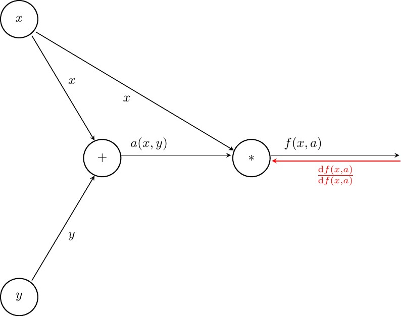
Next we process $f(x,a)$

Then we process $a(x,y)$
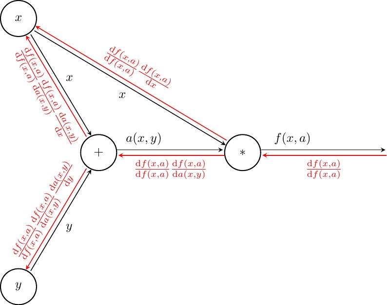
Finally at $x$ and $y$ we perform step 1. of the algorithm to compute $\frac{\mathrm{d}f(x,y)}{\mathrm{d}x}$ and $\frac{\mathrm{d}f(x,y)}{\mathrm{d}y}$
Reconsidering our numeric example from before, were we let $x=2$ and $y=3$, we'd get the following graph
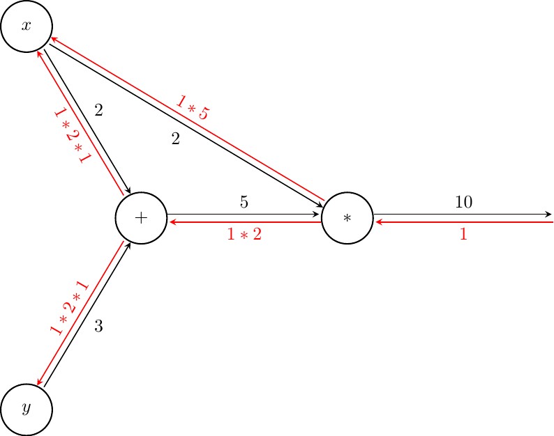
Finally, at $x$ and $y$ we find that $\frac{\mathrm{d}f(x,y)}{\mathrm{d}x}=7$ and $\frac{\mathrm{d}f(x,y)}{\mathrm{d}y}=2$. Mind you that we also know the partial derivatives with respect to $f(x,y)$ for all the intermediate nodes (just the addition in this example).
All it took was visiting each node twice, once when computing the node's output value and once in the backward pass.
What has been presented above is known as reverse automatic differentiation, a technique to numerically evaluate the partial derivatives of a function composed of a set of operations for which isolated partial derivatives are known. Auto differentiation can be executed also in forward mode which won't be covered in this text.
Backpropagation in neural network training refers not only to backpropagating partial derivatives of a loss function with respect to neural weights and biases, but also means application of gradient descent methods to update the parameters accordingly. We will come back to that when doing function optimization.
Summary and Outlook
Up to this point computational graphs (CG) were introduced. A method to compute the value of a CG was presented that used forward propagation of values. Next, a recipe to compute the partial derivatives through backward traversal was given. We've improved the initial formulation by factoring out common terms in what lead to the backpropagation algorithm.
In the a Python library for symbolic and numeric computations will be developed.