28 Ind. Peak Quant

Reads and Mapping Stats:

map_stats=read.csv("../data/comb_map_stats.csv", header=T)
map_stats$line=as.factor(map_stats$line)
map_stats$batch=as.factor(map_stats$batch)

The number of reads for each library and the number of mapped reads.

read_plot=ggplot(map_stats, aes(x=line, y=comb_reads, fill=fraction))+ geom_bar(stat="identity", position="dodge") +labs(y="Reads", title="Reads by line and fraction") 
map_plot=ggplot(map_stats, aes(x=line, y=comb_mapped, fill=fraction))+ geom_bar(stat="identity", position="dodge") +labs(y="Mapped Reads", title="Mapped reads by line and fraction") + geom_hline(yintercept=10000000) + annotate("text",label="10 million mapped reads", y=9000000, x=10)

plot_grid(read_plot, map_plot)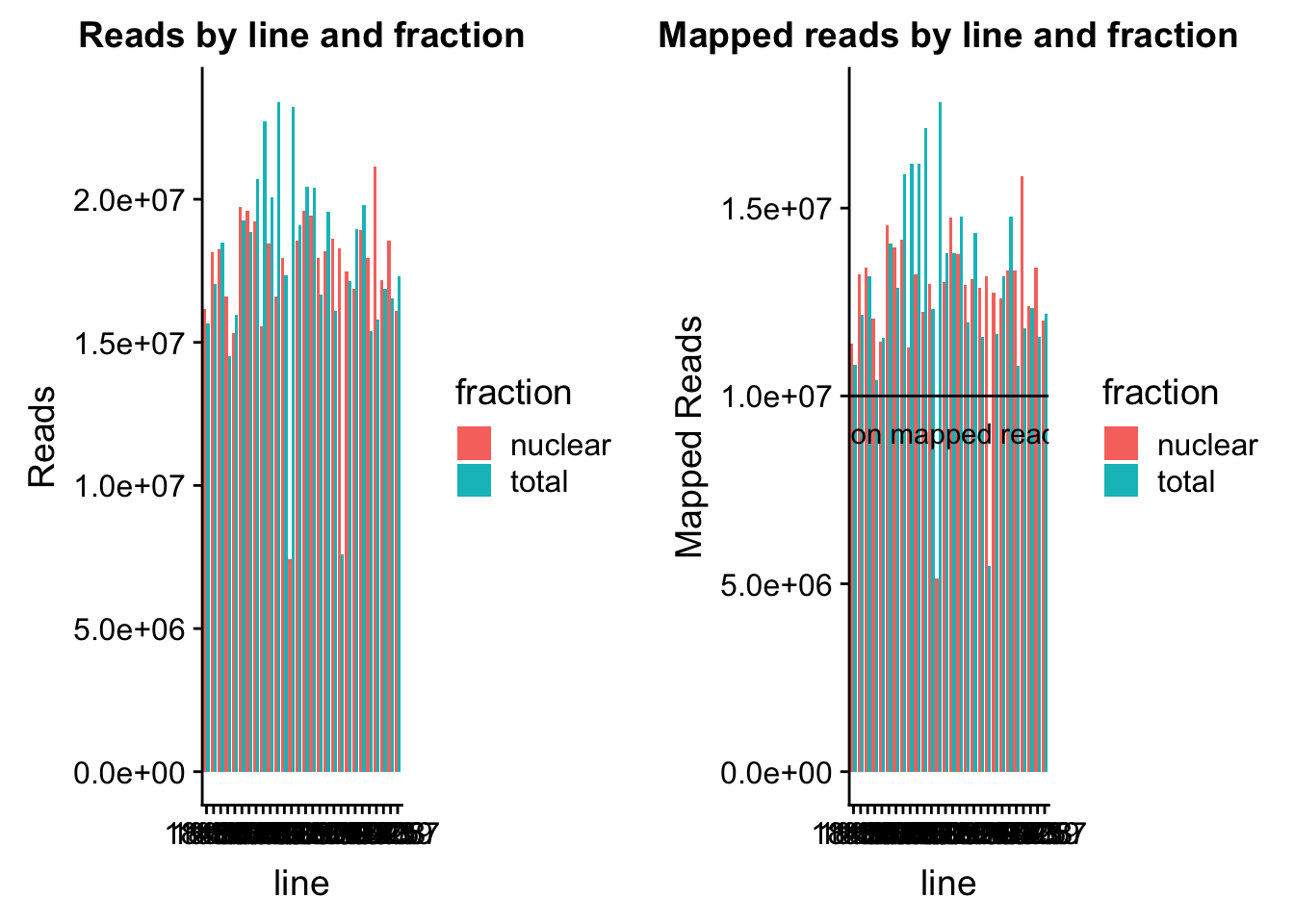

The percent of reads that map per line are pretty uniform accross libraries. The mean is 72%.

ggplot(map_stats, aes(x=line, y=comb_prop_mapped, fill=fraction))+ geom_bar(stat="identity", position="dodge") +labs(y="Mapped Percent", title="Percent of reads mapping by line and fraction")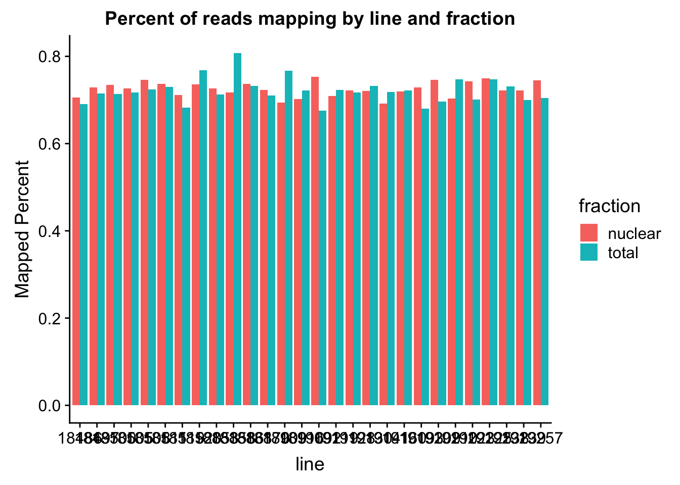 

mean(map_stats$comb_prop_mapped)

[1] 0.7230478

Clean peak exploration

peak_quant=read.table(file = "../data/clean_peaks/APAquant.fc.cleanpeaks.fc", header=T)

Fix the names

file_names=colnames(peak_quant)[7:62]
file_names_split=lapply(file_names, function(x)strsplit(x,".", fixed=T))
libraries=c()
for (i in file_names_split){
  unlist_i=unlist(i)
  libraries=c(libraries, paste(unlist_i[10], unlist_i[11], sep="-"))
}
colnames(peak_quant)=c(colnames(peak_quant)[1:6], libraries)  

Explore the peaks before quantifications:

#length of peaks
plot(sort(peak_quant$Length,decreasing = T), main="Peak Lengths", ylab="Peak Length", xlab="Peak index")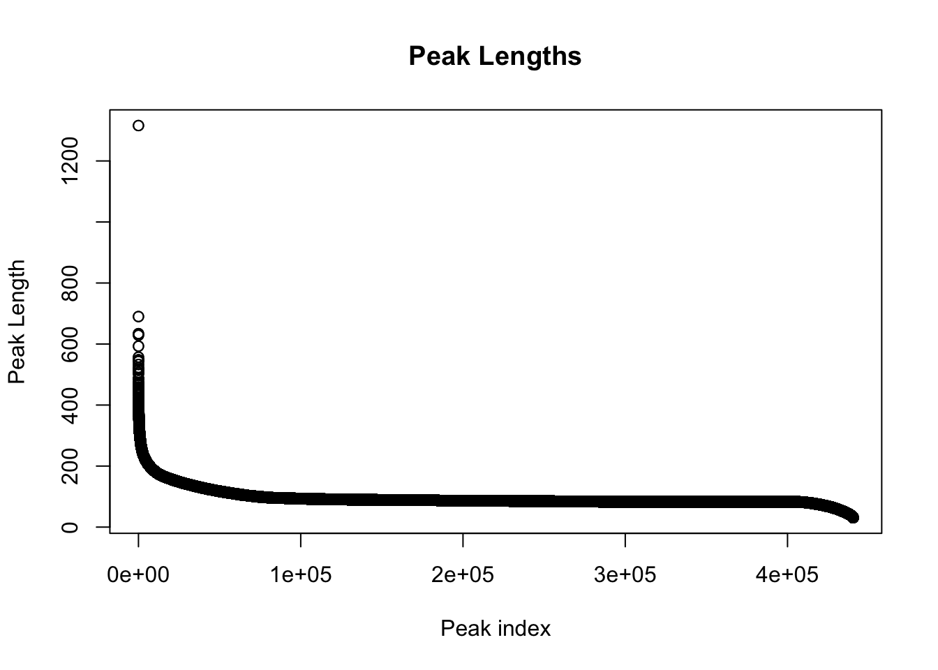

#mean cov of peaks

peak_cov=peak_quant %>% select(contains("-"))

peak_mean=apply(peak_cov,1,mean)
peak_var=apply(peak_cov, 1, var)

plot(log10(sort(peak_mean,decreasing = T)))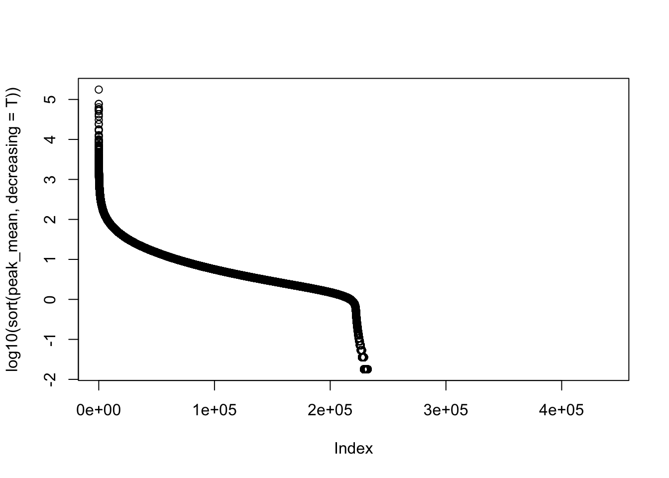

plot(peak_var)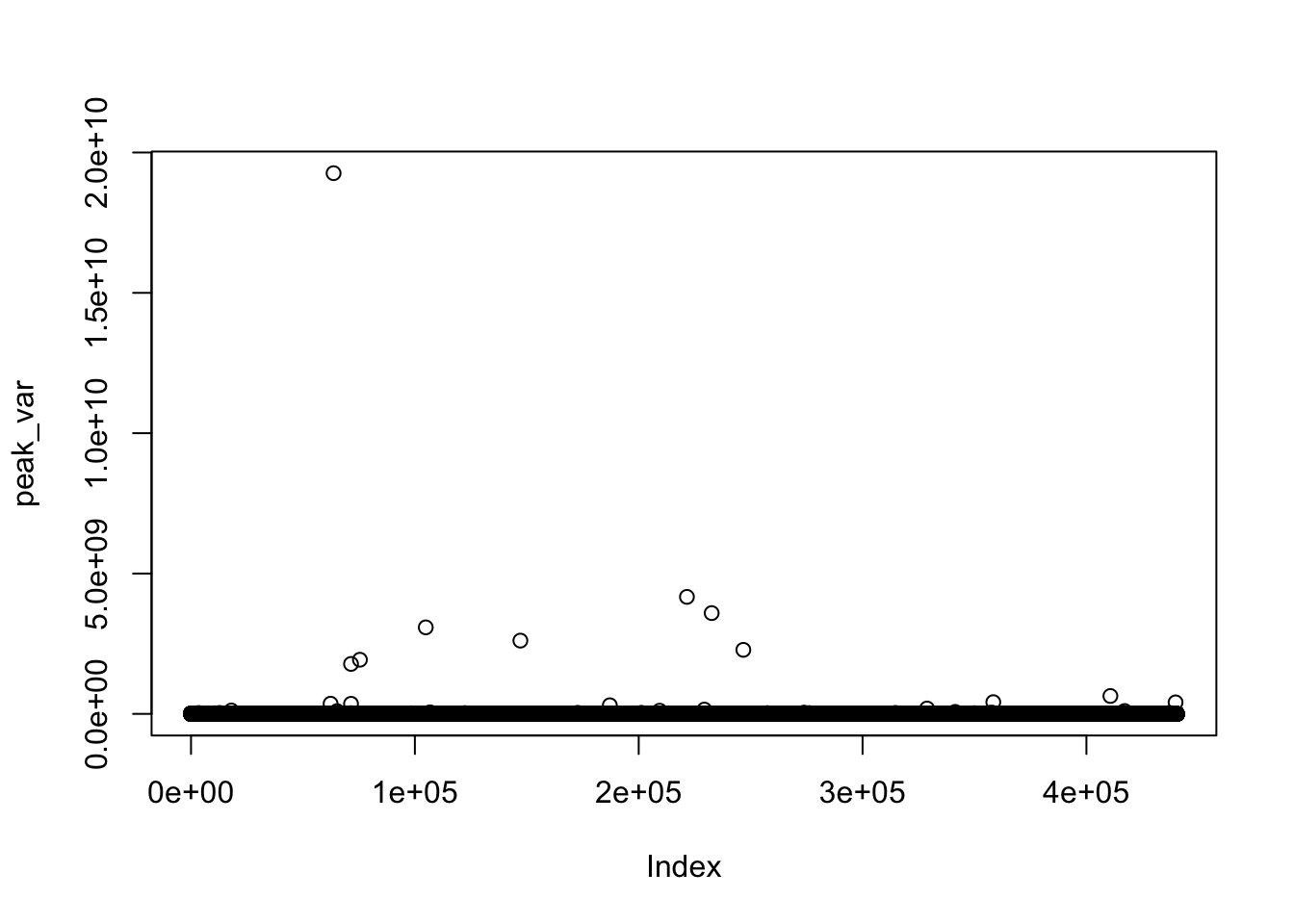

plot(log10(peak_var)~log10(peak_mean))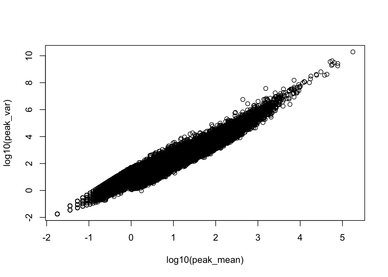

Plot the coverage vs the length:

plot(peak_mean~peak_quant$Length)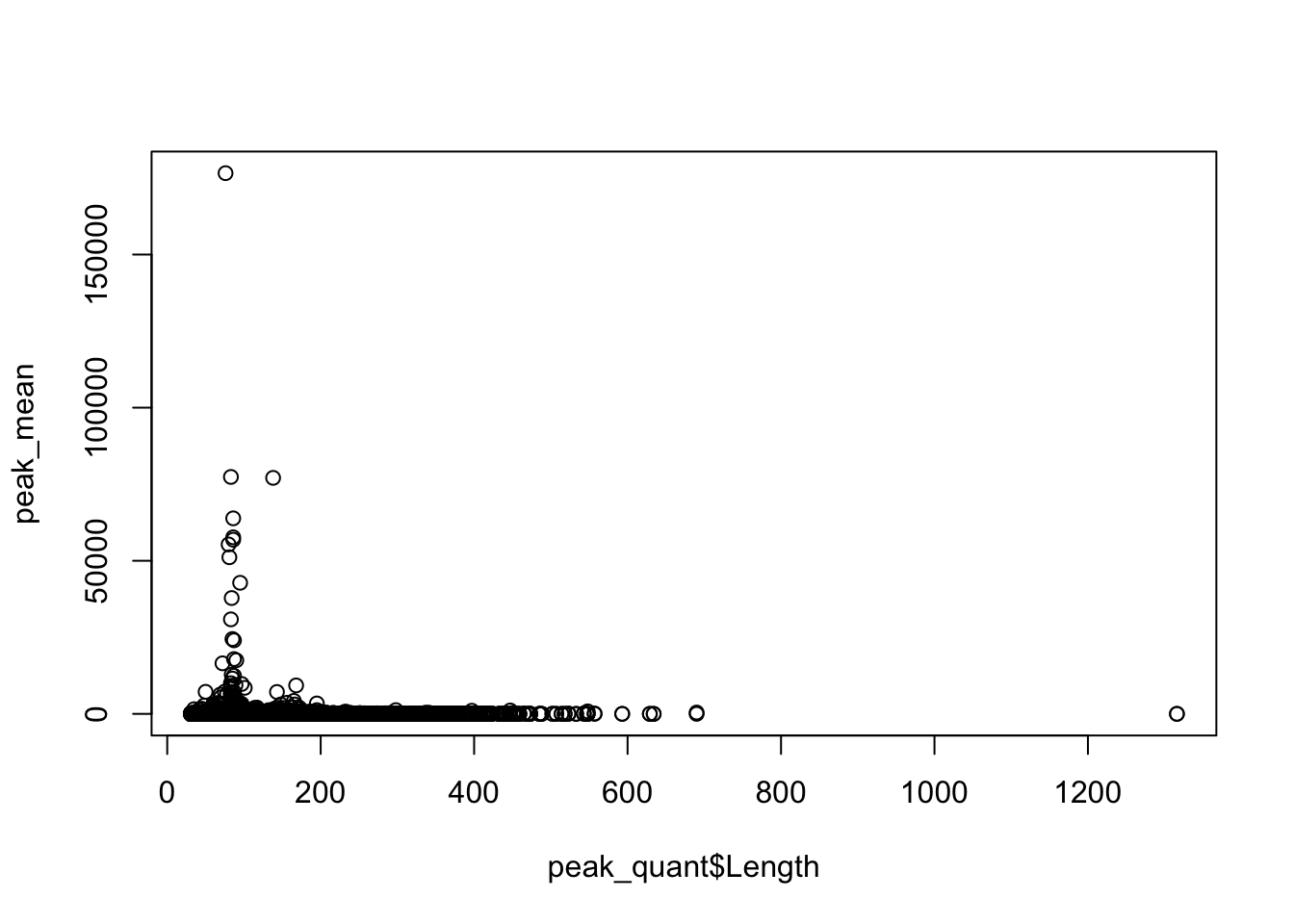

Clustering:

cor_function=function(data){
  corr_matrix= matrix(0,ncol(data),ncol(data))
  for (i in seq(1,ncol(data))){
    for (j in seq(1,ncol(data))){
      x=cor.test(data[,i],  data[,j], method='pearson')
      cor_ij=as.numeric(x$estimate)
      corr_matrix[i,j]=cor_ij
    }
  }
  return(corr_matrix)
}

count_cor=cor_function(peak_cov)
rownames(count_cor)=libraries
colnames(count_cor)=libraries

melted_count_corr=melt(count_cor)
ggheatmap=ggplot(data = melted_count_corr, aes(x=Var1, y=Var2, fill=value)) +
  geom_tile() +
  labs(title="Correlation Heatplot")


ggheatmap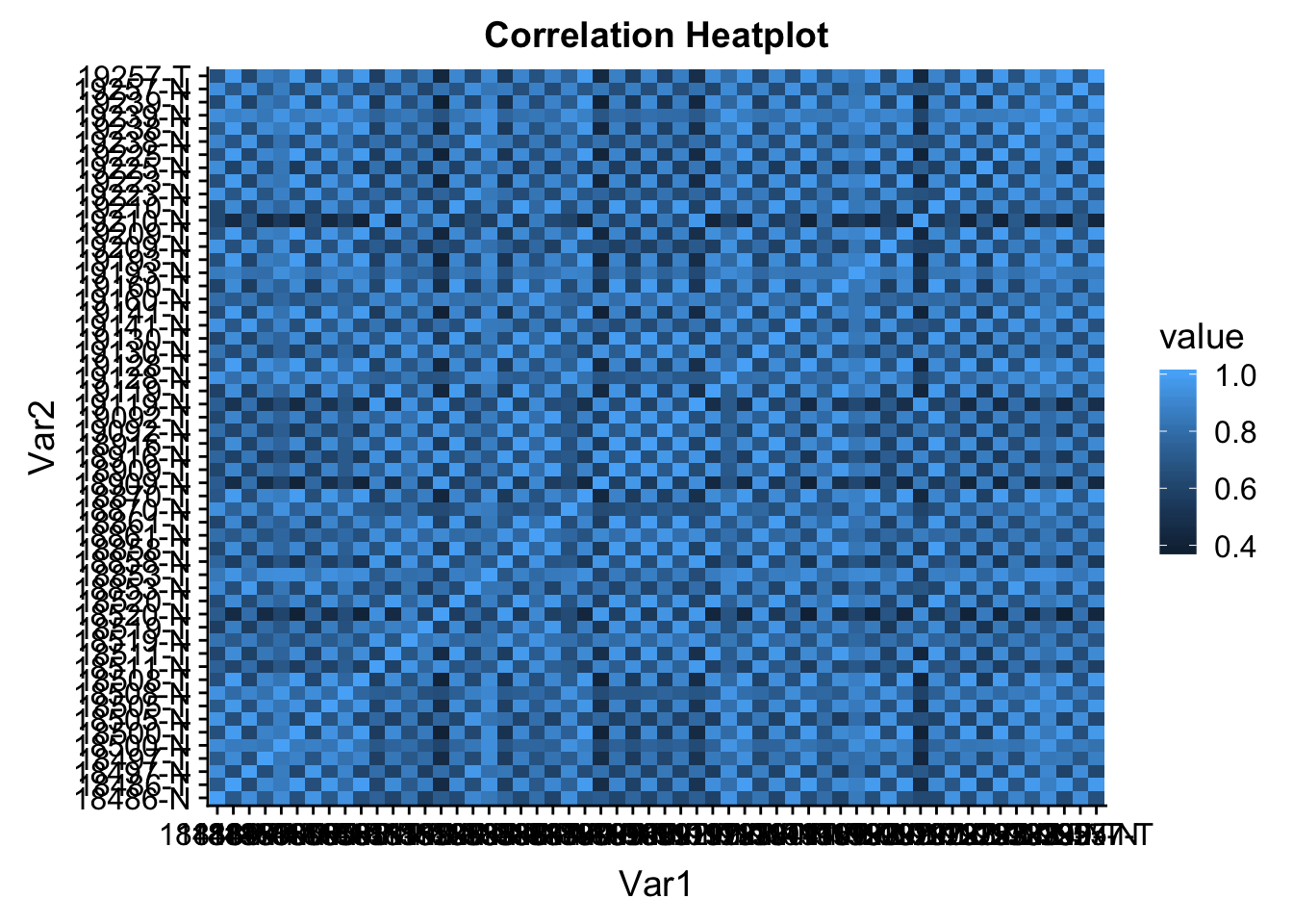

CLustering:

pca_peak= prcomp(peak_cov,center = TRUE,scale. = TRUE)
summary(pca_peak)

Importance of components:
                          PC1    PC2     PC3     PC4    PC5    PC6     PC7
Standard deviation     6.5936 2.7291 1.66983 0.71519 0.6392 0.5651 0.52807
Proportion of Variance 0.7763 0.1330 0.04979 0.00913 0.0073 0.0057 0.00498
Cumulative Proportion  0.7763 0.9093 0.95915 0.96828 0.9756 0.9813 0.98626
                           PC8     PC9    PC10    PC11    PC12    PC13
Standard deviation     0.35808 0.29502 0.25231 0.23732 0.22343 0.19515
Proportion of Variance 0.00229 0.00155 0.00114 0.00101 0.00089 0.00068
Cumulative Proportion  0.98855 0.99010 0.99124 0.99224 0.99314 0.99382
                         PC14    PC15    PC16    PC17    PC18    PC19
Standard deviation     0.1832 0.17407 0.16032 0.14346 0.14122 0.13574
Proportion of Variance 0.0006 0.00054 0.00046 0.00037 0.00036 0.00033
Cumulative Proportion  0.9944 0.99496 0.99542 0.99578 0.99614 0.99647
                         PC20    PC21    PC22    PC23    PC24    PC25
Standard deviation     0.1300 0.12760 0.11966 0.11231 0.10982 0.10799
Proportion of Variance 0.0003 0.00029 0.00026 0.00023 0.00022 0.00021
Cumulative Proportion  0.9968 0.99706 0.99732 0.99754 0.99776 0.99796
                          PC26    PC27    PC28    PC29    PC30    PC31
Standard deviation     0.10167 0.09704 0.09243 0.08607 0.08012 0.07887
Proportion of Variance 0.00018 0.00017 0.00015 0.00013 0.00011 0.00011
Cumulative Proportion  0.99815 0.99832 0.99847 0.99860 0.99872 0.99883
                          PC32    PC33    PC34    PC35    PC36    PC37
Standard deviation     0.07689 0.07601 0.07153 0.06993 0.06656 0.06334
Proportion of Variance 0.00011 0.00010 0.00009 0.00009 0.00008 0.00007
Cumulative Proportion  0.99893 0.99904 0.99913 0.99922 0.99929 0.99937
                          PC38    PC39    PC40    PC41    PC42    PC43
Standard deviation     0.06152 0.05822 0.05643 0.05371 0.05236 0.04715
Proportion of Variance 0.00007 0.00006 0.00006 0.00005 0.00005 0.00004
Cumulative Proportion  0.99943 0.99949 0.99955 0.99960 0.99965 0.99969
                          PC44    PC45    PC46    PC47    PC48    PC49
Standard deviation     0.04656 0.04584 0.04252 0.04214 0.03873 0.03696
Proportion of Variance 0.00004 0.00004 0.00003 0.00003 0.00003 0.00002
Cumulative Proportion  0.99973 0.99977 0.99980 0.99983 0.99986 0.99988
                          PC50    PC51    PC52    PC53    PC54    PC55
Standard deviation     0.03557 0.03351 0.03191 0.03020 0.02938 0.02733
Proportion of Variance 0.00002 0.00002 0.00002 0.00002 0.00002 0.00001
Cumulative Proportion  0.99991 0.99993 0.99994 0.99996 0.99998 0.99999
                          PC56
Standard deviation     0.02525
Proportion of Variance 0.00001
Cumulative Proportion  1.00000

pc_df=as.data.frame(pca_peak$rotation) %>% rownames_to_column(var="lib") %>% mutate(fraction=ifelse(grepl("T", lib), "total", "nuclear"))

ggplot(pc_df, aes(x=PC1, y=PC2, col=fraction)) + geom_point() + labs(x="PC1: Prop explained 0.7763", y="PC2: Prop explained 0.1330", title="Raw PAS qunatification data")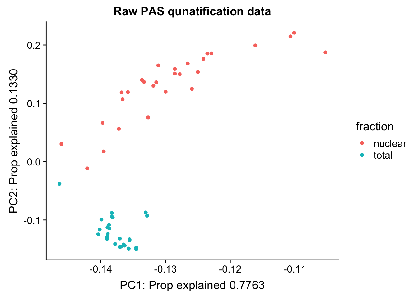

I now want to explore what the first PC is representing. Some ideas are:

• batch

• sequencing depth

• mapped reads

All of this info is in the map stats.

pc_df=as.data.frame(pca_peak$rotation) %>% rownames_to_column(var="lib") %>% mutate(fraction=ifelse(grepl("T", lib), "total", "nuclear")) %>% mutate(reads=map_stats$comb_reads) %>% mutate(batch=map_stats$batch) %>% mutate(mapped=map_stats$comb_mapped)


batch_gg= ggplot(pc_df, aes(x=PC1, y=PC2, col=batch)) + geom_point() + labs(x="PC1: Prop explained 0.7763", y="PC2: Prop explained 0.1330", title="Batch")

frac_gg= ggplot(pc_df, aes(x=PC1, y=PC2, col=fraction)) + geom_point() + labs(x="PC1: Prop explained 0.7763", y="PC2: Prop explained 0.1330", title="Fraction")

reads_gg= ggplot(pc_df, aes(x=PC1, y=PC2, col=reads)) + geom_point() + labs(x="PC1: Prop explained 0.7763", y="PC2: Prop explained 0.1330", title="Reads")


mapped_gg= ggplot(pc_df, aes(x=PC1, y=PC2, col=mapped)) + geom_point() + labs(x="PC1: Prop explained 0.7763", y="PC2: Prop explained 0.1330", title="Mapped Reads")

plot_grid(frac_gg,batch_gg,reads_gg,mapped_gg)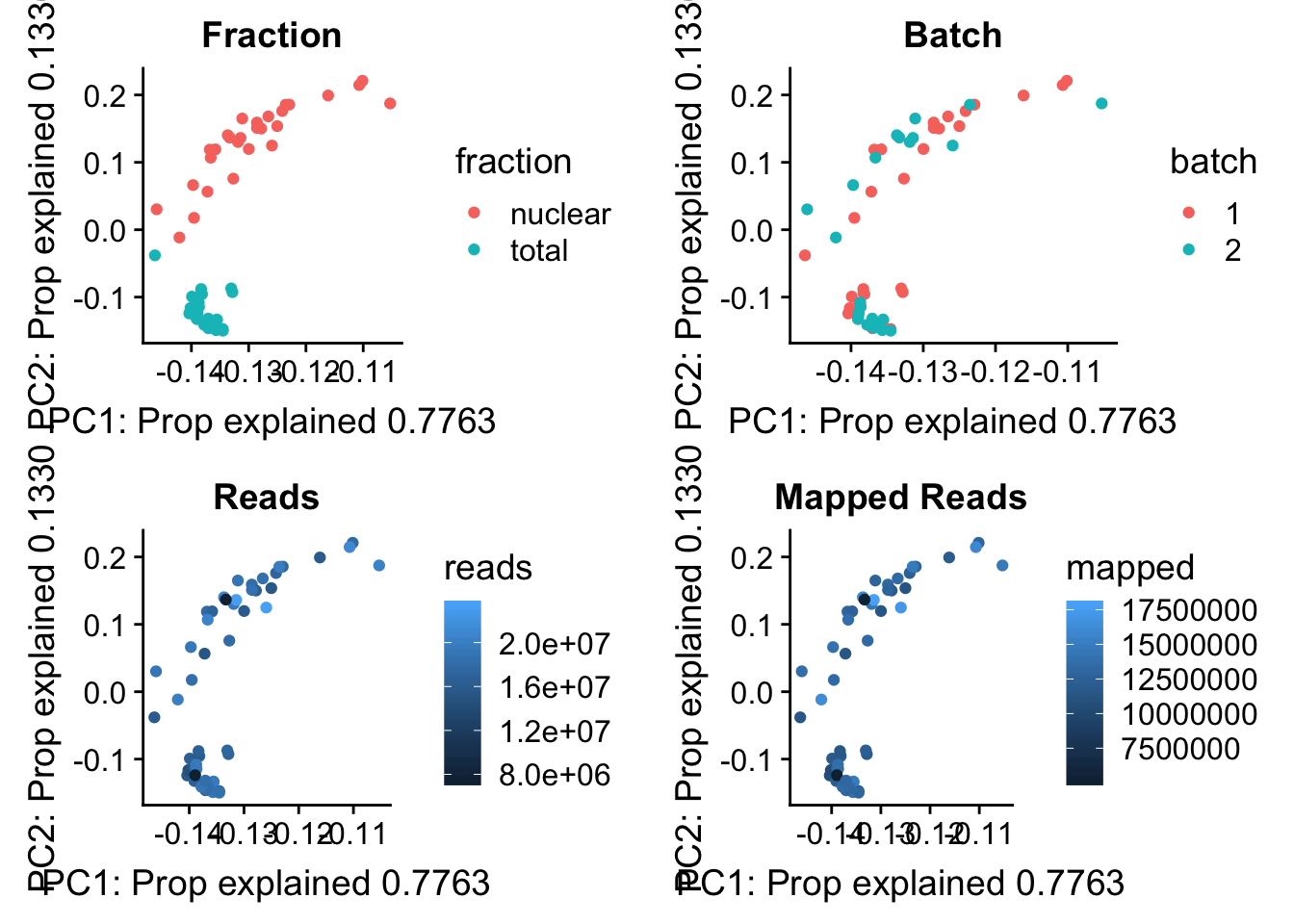

Proportion of reads mapping to peaks. This may be in the feature counts summary.

Session information

sessionInfo()

R version 3.5.1 (2018-07-02)
Platform: x86_64-apple-darwin15.6.0 (64-bit)
Running under: macOS Sierra 10.12.6

Matrix products: default
BLAS: /Library/Frameworks/R.framework/Versions/3.5/Resources/lib/libRblas.0.dylib
LAPACK: /Library/Frameworks/R.framework/Versions/3.5/Resources/lib/libRlapack.dylib

locale:
[1] en_US.UTF-8/en_US.UTF-8/en_US.UTF-8/C/en_US.UTF-8/en_US.UTF-8

attached base packages:
[1] stats     graphics  grDevices utils     datasets  methods   base     

other attached packages:
 [1] bindrcpp_0.2.2  devtools_1.13.6 reshape2_1.4.3  cowplot_0.9.3  
 [5] workflowr_1.1.1 forcats_0.3.0   stringr_1.3.1   dplyr_0.7.6    
 [9] purrr_0.2.5     readr_1.1.1     tidyr_0.8.1     tibble_1.4.2   
[13] ggplot2_3.0.0   tidyverse_1.2.1

loaded via a namespace (and not attached):
 [1] tidyselect_0.2.4  haven_1.1.2       lattice_0.20-35  
 [4] colorspace_1.3-2  htmltools_0.3.6   yaml_2.1.19      
 [7] rlang_0.2.1       R.oo_1.22.0       pillar_1.3.0     
[10] glue_1.3.0        withr_2.1.2       R.utils_2.6.0    
[13] modelr_0.1.2      readxl_1.1.0      bindr_0.1.1      
[16] plyr_1.8.4        munsell_0.5.0     gtable_0.2.0     
[19] cellranger_1.1.0  rvest_0.3.2       R.methodsS3_1.7.1
[22] memoise_1.1.0     evaluate_0.11     labeling_0.3     
[25] knitr_1.20        broom_0.5.0       Rcpp_0.12.18     
[28] backports_1.1.2   scales_0.5.0      jsonlite_1.5     
[31] hms_0.4.2         digest_0.6.15     stringi_1.2.4    
[34] grid_3.5.1        rprojroot_1.3-2   cli_1.0.0        
[37] tools_3.5.1       magrittr_1.5      lazyeval_0.2.1   
[40] crayon_1.3.4      whisker_0.3-2     pkgconfig_2.0.1  
[43] xml2_1.2.0        lubridate_1.7.4   assertthat_0.2.0 
[46] rmarkdown_1.10    httr_1.3.1        rstudioapi_0.7   
[49] R6_2.2.2          nlme_3.1-137      git2r_0.23.0     
[52] compiler_3.5.1