Quantify reads per Peaks
Briana Mittleman
8/24/2018
Last updated: 2018-08-27
workflowr checks: (Click a bullet for more information)-
✔ R Markdown file: up-to-date
Great! Since the R Markdown file has been committed to the Git repository, you know the exact version of the code that produced these results.
-
✔ Environment: empty
Great job! The global environment was empty. Objects defined in the global environment can affect the analysis in your R Markdown file in unknown ways. For reproduciblity it’s best to always run the code in an empty environment.
-
✔ Seed:
set.seed(20180801)The command
set.seed(20180801)was run prior to running the code in the R Markdown file. Setting a seed ensures that any results that rely on randomness, e.g. subsampling or permutations, are reproducible. -
✔ Session information: recorded
Great job! Recording the operating system, R version, and package versions is critical for reproducibility.
-
Great! You are using Git for version control. Tracking code development and connecting the code version to the results is critical for reproducibility. The version displayed above was the version of the Git repository at the time these results were generated.✔ Repository version: 2bcaafd
Note that you need to be careful to ensure that all relevant files for the analysis have been committed to Git prior to generating the results (you can usewflow_publishorwflow_git_commit). workflowr only checks the R Markdown file, but you know if there are other scripts or data files that it depends on. Below is the status of the Git repository when the results were generated:
Note that any generated files, e.g. HTML, png, CSS, etc., are not included in this status report because it is ok for generated content to have uncommitted changes.Ignored files: Ignored: .RData Ignored: .Rhistory Ignored: .Rproj.user/ Untracked files: Untracked: com_threeprime.Rproj Untracked: data/PeakPerExon/ Untracked: data/PeakPerGene/ Untracked: data/comp.pheno.data.csv Untracked: data/dist_TES/ Untracked: data/dist_upexon/ Untracked: data/liftover/ Untracked: data/map.stats.csv Untracked: data/map.stats.xlsx Untracked: data/orthoPeak_quant/ Unstaged changes: Deleted: comparitive_threeprime.Rproj
Expand here to see past versions:
| File | Version | Author | Date | Message |
|---|---|---|---|---|
| html | 2bcaafd | brimittleman | 2018-08-27 | Build site. |
| html | 6680d6f | brimittleman | 2018-08-27 | Build site. |
| Rmd | bb29739 | brimittleman | 2018-08-27 | norm and filter |
| html | 5049ea1 | brimittleman | 2018-08-27 | Build site. |
| Rmd | 686bab0 | brimittleman | 2018-08-27 | rpm |
| html | b9db900 | brimittleman | 2018-08-24 | Build site. |
| Rmd | 489ba43 | brimittleman | 2018-08-24 | think about normalize options |
| html | 0c5a4d1 | brimittleman | 2018-08-24 | Build site. |
| Rmd | 32a9409 | brimittleman | 2018-08-24 | compare raw to cpm |
| html | bc94507 | brimittleman | 2018-08-24 | Build site. |
| Rmd | 189a2fb | brimittleman | 2018-08-24 | organize |
| html | d0e92f5 | brimittleman | 2018-08-24 | Build site. |
| Rmd | 43f6773 | brimittleman | 2018-08-24 | prenormalization PCA |
| html | 5b4893e | brimittleman | 2018-08-24 | Build site. |
| Rmd | 679aef4 | brimittleman | 2018-08-24 | initalize reads per peak analysis and update index |
Feature count
In this analysis I will run feature counts on the human and chimp,total and nuclear threeprime seq libraries agaisnt the orthologous peaks I called with liftover.
First I will need to convert the bed files to saf files. This File is GeneID, Chr, Start, End, Strand. In my case it is peak ID.
#human
from misc_helper import *

fout = file("/project2/gilad/briana/comparitive_threeprime/data/ortho_peaks/humanOrthoPeaks.sort.SAF",'w')
fout.write("GeneID\tChr\tStart\tEnd\tStrand\n")
for ln in open("/project2/gilad/briana/comparitive_threeprime/data/ortho_peaks/humanOrthoPeaks.sort.bed"):
    chrom, start, end, name = ln.split()
    start=int(start)
    end=int(end)
    fout.write("%s\t%s\t%d\t%d\t.\n"%(name, chrom, start, end))

fout.close()


#chimp
from misc_helper import *

fout = file("/project2/gilad/briana/comparitive_threeprime/data/ortho_peaks/chimpOrthoPeaks.sort.SAF",'w')
fout.write("GeneID\tChr\tStart\tEnd\tStrand\n")
for ln in open("/project2/gilad/briana/comparitive_threeprime/data/ortho_peaks/chimpOrthoPeaks.sort.bed"):
    chrom, start, end, name = ln.split()
    start=int(start)
    end=int(end)
    fout.write("%s\t%s\t%d\t%d\t.\n"%(name, chrom, start, end))

fout.close()
The resulting files are:
/project2/gilad/briana/comparitive_threeprime/data/ortho_peaks/chimpOrthoPeaks.sort.saf
/project2/gilad/briana/comparitive_threeprime/data/ortho_peaks/humanOrthoPeaks.sort.saf
#!/bin/bash

#SBATCH --job-name=fc_orthopeaks
#SBATCH --account=pi-yangili1
#SBATCH --time=24:00:00
#SBATCH --output=fc_orthopeaks.out
#SBATCH --error=fc_orthopeaks.err
#SBATCH --partition=broadwl
#SBATCH --mem=12G
#SBATCH --mail-type=END


module load Anaconda3
source activate comp_threeprime_env

# outdir: /project2/gilad/briana/comparitive_threeprime/data/Peak_quant

#-s 0 is unstranded

featureCounts -a /project2/gilad/briana/comparitive_threeprime/data/ortho_peaks/humanOrthoPeaks.sort.SAF -F SAF -o /project2/gilad/briana/comparitive_threeprime/data/Peak_quant/HumanTotal_Orthopeak.quant /project2/gilad/briana/comparitive_threeprime/human/data/sort/*T-sort.bam -s 0

featureCounts -a /project2/gilad/briana/comparitive_threeprime/data/ortho_peaks/humanOrthoPeaks.sort.SAF -F SAF -o /project2/gilad/briana/comparitive_threeprime/data/Peak_quant/HumanNuclear_Orthopeak.quant /project2/gilad/briana/comparitive_threeprime/human/data/sort/*N-sort.bam -s 0


featureCounts -a /project2/gilad/briana/comparitive_threeprime/data/ortho_peaks/chimpOrthoPeaks.sort.SAF -F SAF -o /project2/gilad/briana/comparitive_threeprime/data/Peak_quant/ChimpTotal_Orthopeak.quant /project2/gilad/briana/comparitive_threeprime/chimp/data/sort/*T-sort.bam -s 0

featureCounts -a /project2/gilad/briana/comparitive_threeprime/data/ortho_peaks/chimpOrthoPeaks.sort.SAF -F SAF -o /project2/gilad/briana/comparitive_threeprime/data/Peak_quant/ChimpNuclear_Orthopeak.quant /project2/gilad/briana/comparitive_threeprime/chimp/data/sort/*N-sort.bam -s 0
Visualize raw counts
I need the matching peaks from human and chimps from the liftover pipeline data.
library(workflowr)This is workflowr version 1.1.1
Run ?workflowr for help getting startedlibrary(tidyverse)── Attaching packages ─────────────────────────────────────────────────── tidyverse 1.2.1 ──✔ ggplot2 3.0.0 ✔ purrr 0.2.5
✔ tibble 1.4.2 ✔ dplyr 0.7.6
✔ tidyr 0.8.1 ✔ stringr 1.3.1
✔ readr 1.1.1 ✔ forcats 0.3.0── Conflicts ────────────────────────────────────────────────────── tidyverse_conflicts() ──
✖ dplyr::filter() masks stats::filter()
✖ dplyr::lag() masks stats::lag()library(reshape2)
Attaching package: 'reshape2'The following object is masked from 'package:tidyr':
smithslibrary(cowplot)
Attaching package: 'cowplot'The following object is masked from 'package:ggplot2':
ggsavePeakNames=read.table(file = "../data/liftover/HumanChimpPeaknames.txt", header=T, stringsAsFactors = F)Chimps:
- 18358
- 3622
- 3659
- 4973
- pt30
- pt91
Humans:
- 18498
- 18499
- 18502
- 18504
- 18510
- 18523
namesHN= c("human","Chr", "Start", "End", "Strand", "Length", "N18498", "N18499", "N18502", "N18504", "N18510", "N18523")
humanNuc=read.table("../data/orthoPeak_quant/HumanNuclear_Orthopeak.quant", header = T, stringsAsFactors = F, col.names = namesHN)

namesHT= c("human","Chr", "Start", "End", "Strand", "Length", "T18498", "T18499", "T18502", "T18504", "T18510", "T18523")
humanTot=read.table("../data/orthoPeak_quant/HumanTotal_Orthopeak.quant", header=T, stringsAsFactors = F, col.names = namesHT)


namesCN= c("chimp","Chr", "Start", "End", "Strand", "Length", "N18358", "N3622", "N3659", "N4973", "Npt30", "Npt91")

chimpNuc=read.table("../data/orthoPeak_quant/ChimpNuclear_Orthopeak.quant", header = T,stringsAsFactors = F, col.names = namesCN)

namesCT= c("chimp","Chr", "Start", "End", "Strand", "Length", "T18358", "T3622", "T3659", "T4973", "Tpt30", "Tpt91")
chimpTot=read.table("../data/orthoPeak_quant/ChimpTotal_Orthopeak.quant", header=T, stringsAsFactors = F, col.names = namesCT)
I need to add the human names to the chimp file and chimp names to the human files.
humanNuc_ed= humanNuc %>% inner_join(PeakNames, by="human") %>% mutate(ID=paste(human,chimp, sep=":")) %>% select("ID",  "N18498", "N18499", "N18502", "N18504", "N18510", "N18523")

humanTot_ed= humanTot %>% inner_join(PeakNames, by="human") %>%mutate(ID=paste(human,chimp, sep=":")) %>% select("ID",  "T18498", "T18499", "T18502", "T18504", "T18510", "T18523")

chimpNuc_ed=chimpNuc %>% inner_join(PeakNames, by="chimp") %>% mutate(ID=paste(human,chimp, sep=":")) %>% select("ID", "N18358", "N3622", "N3659", "N4973", "Npt30", "Npt91")

chimpTot_ed= chimpTot %>% inner_join(PeakNames, by="chimp") %>% mutate(ID=paste(human,chimp, sep=":")) %>% select("ID", "T18358", "T3622", "T3659", "T4973", "Tpt30", "Tpt91")
Now I need to join all of these together by the peaks.
allPeakQuant= humanNuc_ed %>% left_join(humanTot_ed, by="ID") %>% left_join(chimpNuc_ed, by="ID") %>% left_join(chimpTot_ed, by="ID") %>% column_to_rownames(var="ID")
allPeakQuant_matrix=as.matrix(allPeakQuant)
Run PCA:
humans=c("N18498", "N18499", "N18502", "N18504", "N18510", "N18523", "T18498", "T18499", "T18502", "T18504", "T18510", "T18523")
pc=prcomp(allPeakQuant_matrix)
rotation=data.frame(pc$rotation) %>% rownames_to_column(var="Sample") %>% mutate(Fraction=ifelse(grepl("N", Sample), "Nuclear", "Total")) %>% mutate(Species= ifelse(Sample %in% humans, "Human", "Chimp"))
Plot this:
prenormPCA=ggplot(rotation, aes(x=PC1, y=PC2, col=Species, shape=Fraction)) + geom_point() + labs(title="Prenormalization PCA")

prenormPCA34=ggplot(rotation, aes(x=PC3, y=PC4, col=Species, shape=Fraction)) + geom_point() + labs(title="Prenormalization PCA")

prenormPCA56=ggplot(rotation, aes(x=PC5, y=PC6, col=Species, shape=Fraction)) + geom_point() + labs(title="Prenormalization PCA")

prenormPCA78=ggplot(rotation, aes(x=PC7, y=PC8, col=Species, shape=Fraction)) + geom_point() + labs(title="Prenormalization PCA")
plot_grid(prenormPCA,prenormPCA34, prenormPCA56, prenormPCA78)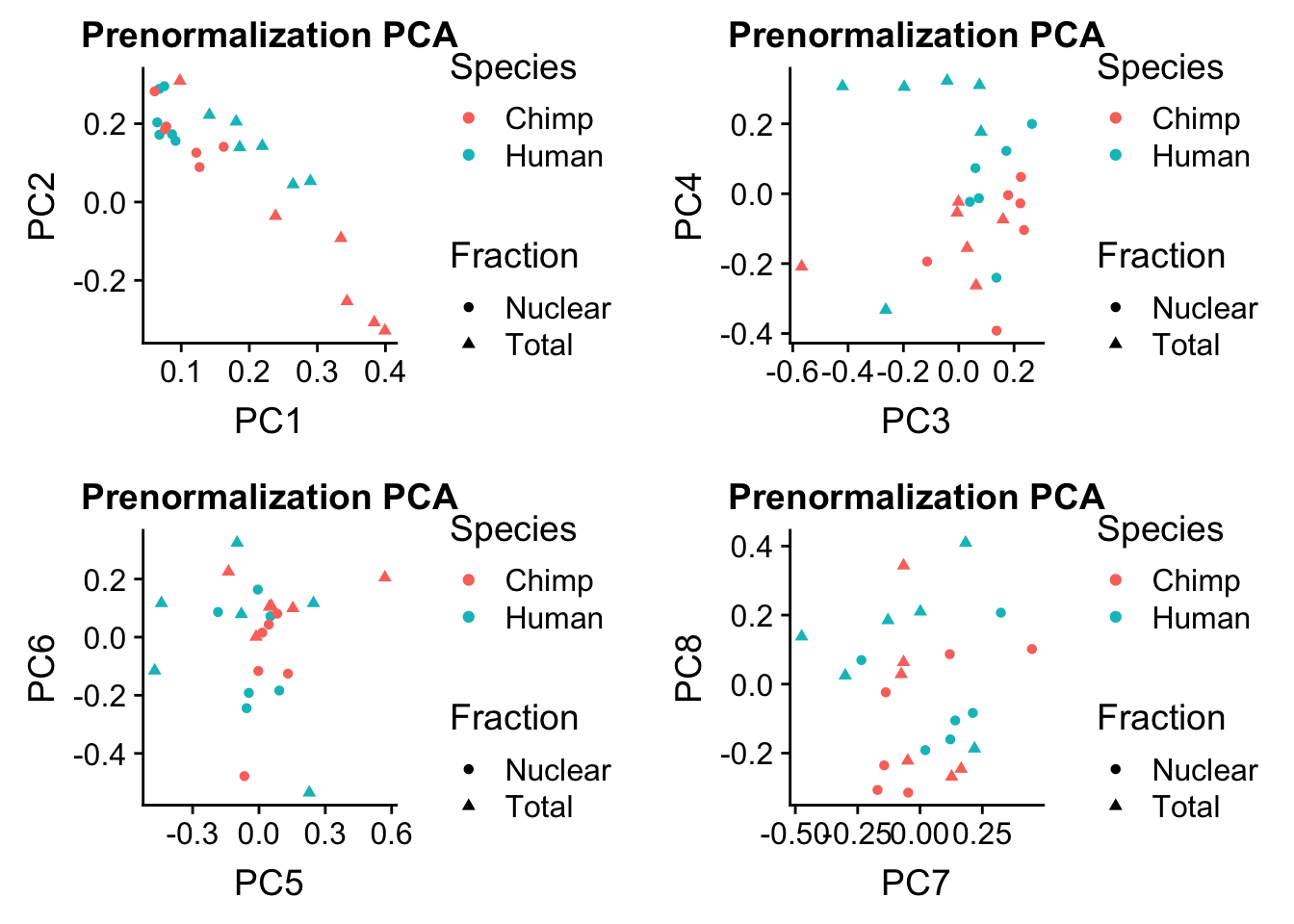
Expand here to see past versions of unnamed-chunk-10-1.png:
| Version | Author | Date |
|---|---|---|
| d0e92f5 | brimittleman | 2018-08-24 |
Normalize counts
To normalize this i will need to understand the distributions. I am not sure if this data will be normal.
library(edgeR)Loading required package: limmaallPeakQuant_matrix_cpm=cpm(allPeakQuant_matrix, log=T)
plotDensities(allPeakQuant_matrix_cpm, legend = "bottomright", main="Pre-filtering")
abline(v = 0, lty = 3)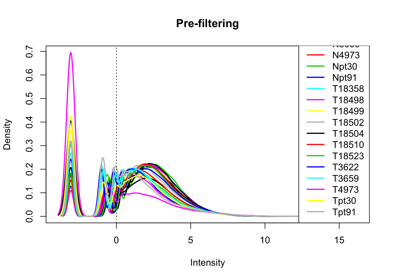
Expand here to see past versions of unnamed-chunk-12-1.png:
| Version | Author | Date |
|---|---|---|
| 0c5a4d1 | brimittleman | 2018-08-24 |
par(mfrow=c(2,1))
boxplot(log10(allPeakQuant + 1), main="Log Raw Counts + 1")
boxplot(allPeakQuant_matrix_cpm, main="Log CPM Counts")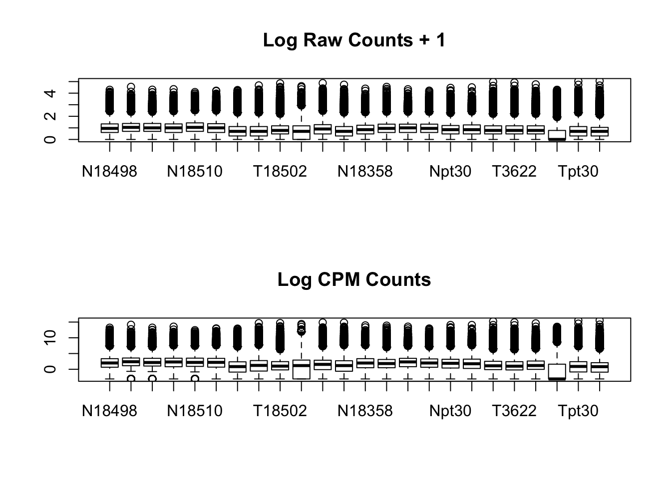
Expand here to see past versions of unnamed-chunk-13-1.png:
| Version | Author | Date |
|---|---|---|
| 0c5a4d1 | brimittleman | 2018-08-24 |
I should think about other normalization types. I am going to look at other papers to see what they do. For example, Derti et al. 2012.
“All samples were normalized to equal numbers of aligned sequencing reads by random selection”
Things to think about:
peak size diff in human/chimp
divide by lib size or mapped reads or reads mapping to peaks
From Wang et al. 2018
reads per million for all samples (RPM)
percent of samples with expression (PSE)
mean RPM and PSE of each isoform normalzied by summed RPM and max PSE of all isoforms of the corresponding gene (relative abundance and normalzied PSE)
PAS expressed in sample if >2 reads per sample
diversity - Shannon Index \(D=\sum^{S}_{i=1}p_{i}lnp_{i}\) where \(p_{i}\) is the relative usage of the ith PAS for a given gene with S number of PAS
I will compute the PRM for the matrix using the library read counts.
read_stats=read.csv("../data/map.stats.csv", header = T) %>% mutate(library=paste(substr(Fraction,1,1), Line, sep="")) %>% select(library, Reads)I want to divide the values in the column corresponding to a specific library by the value in the Reads columns in the map_stats. I will use for loops for now (should use apply)
allPeakQuant_matrix_rpm=as.data.frame(matrix("NA", nrow = nrow(allPeakQuant_matrix), ncol=ncol(allPeakQuant_matrix)))
colnames(allPeakQuant_matrix_rpm)=colnames(allPeakQuant_matrix)
rownames(allPeakQuant_matrix_rpm)=rownames(allPeakQuant_matrix)

library_order=order(read_stats$library)

allPeakQuant_matrix_rpm=allPeakQuant_matrix_rpm[,order(library_order)]
allPeakQuant_matrix=allPeakQuant_matrix[,order(library_order)]
read_stats_T=read_stats%>% t


#filter for more than 2 reads
allPeakQuant_matrix_filt=ifelse(allPeakQuant_matrix<=2,0,allPeakQuant_matrix)


#make RPM
for (i in seq(1:ncol(allPeakQuant_matrix))) {
  x=as.integer(read_stats_T[2,i])/1000000
  allPeakQuant_matrix_rpm[,i]=as.vector(allPeakQuant_matrix_filt[,i])/x
}
par(mfrow=c(2,1))
boxplot(log10(allPeakQuant + 1), main="Log Raw Counts + 1")
boxplot(log10(allPeakQuant_matrix_rpm + 1), main="log 10 RPM Counts + 1")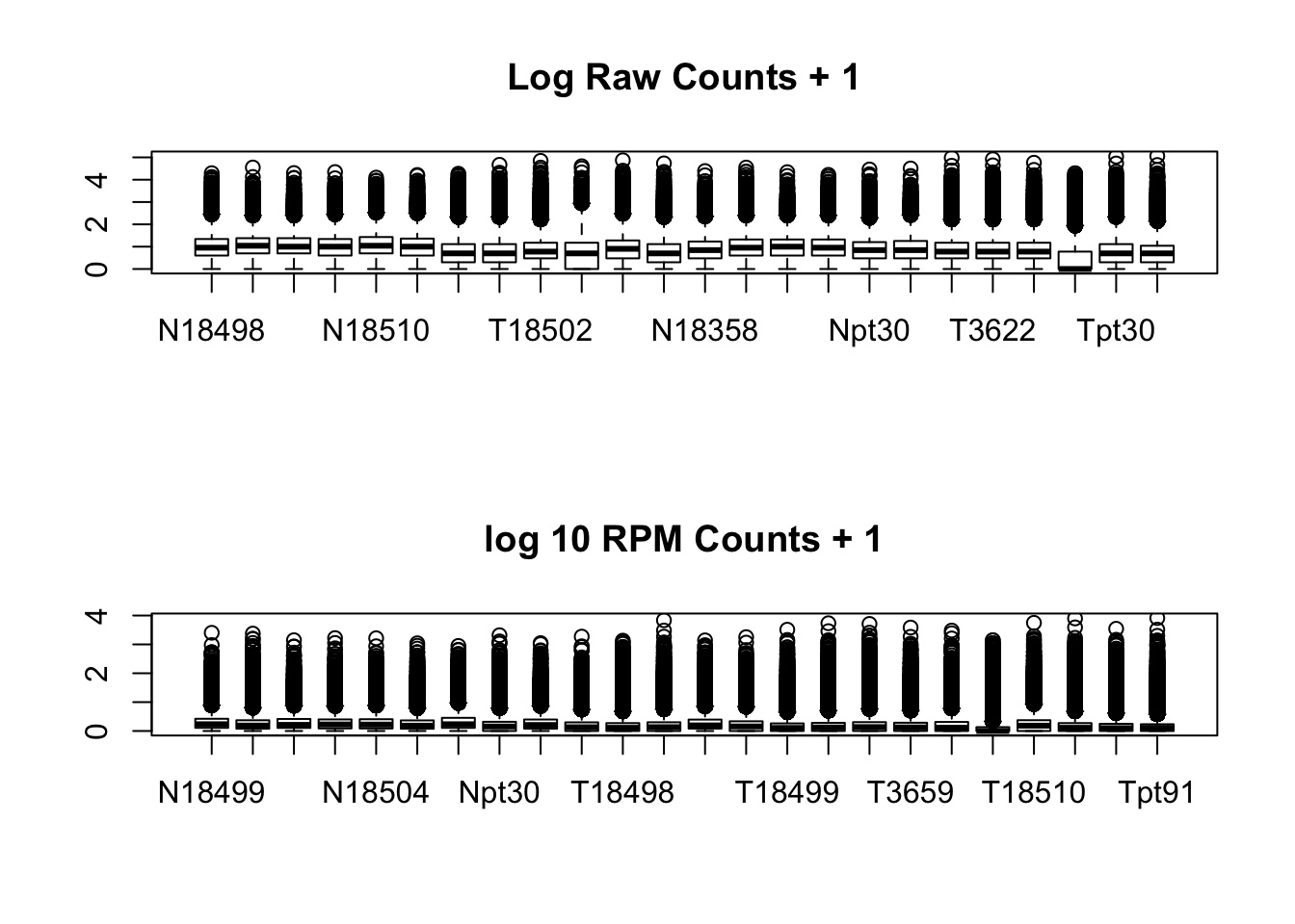
Expand here to see past versions of unnamed-chunk-16-1.png:
| Version | Author | Date |
|---|---|---|
| 6680d6f | brimittleman | 2018-08-27 |
| 5049ea1 | brimittleman | 2018-08-27 |
plotDensities(log10(allPeakQuant_matrix_rpm+1), legend = "bottomright", main="RPM")
abline(v = 0, lty = 3)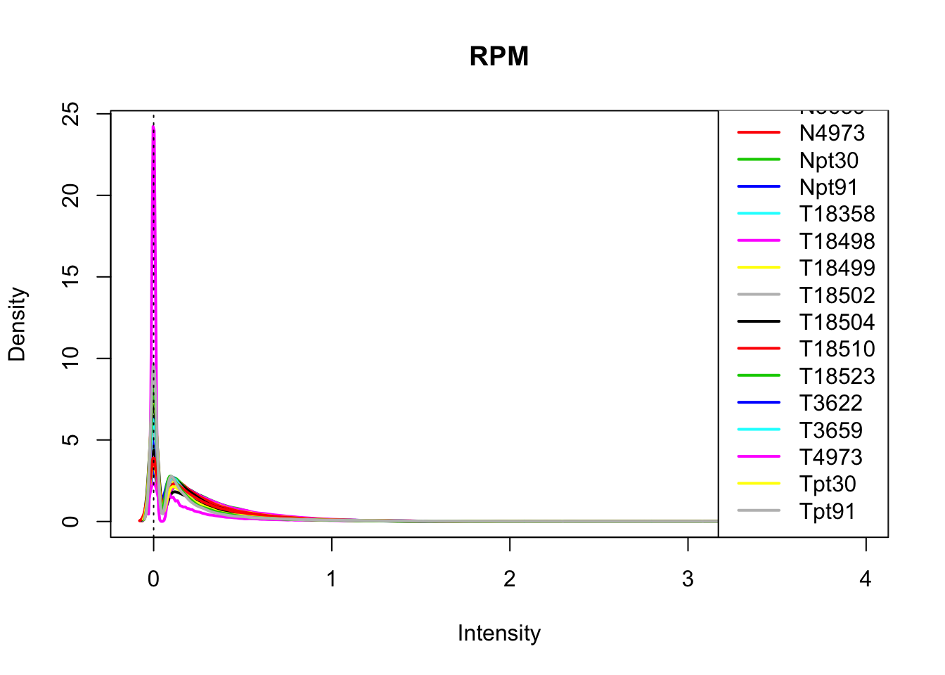
Expand here to see past versions of unnamed-chunk-17-1.png:
| Version | Author | Date |
|---|---|---|
| 6680d6f | brimittleman | 2018-08-27 |
| 5049ea1 | brimittleman | 2018-08-27 |
Normalize by the sample RPM average for each sample:
RPM_mean=apply(allPeakQuant_matrix_rpm, 2,function(x)mean(x))


allPeakQuant_matrix_rpm_Norm=allPeakQuant_matrix_rpm


for (i in seq(1:ncol(allPeakQuant_matrix_rpm_Norm))) {
  allPeakQuant_matrix_rpm_Norm[,i]=as.vector(allPeakQuant_matrix_rpm[,i])/RPM_mean[i]
}
par(mfrow=c(2,1))
boxplot(log10(allPeakQuant + 1), main="Log Raw Counts + 1")
boxplot(log10(allPeakQuant_matrix_rpm_Norm + 1), main="Normalized log 10 RPM Counts + 1")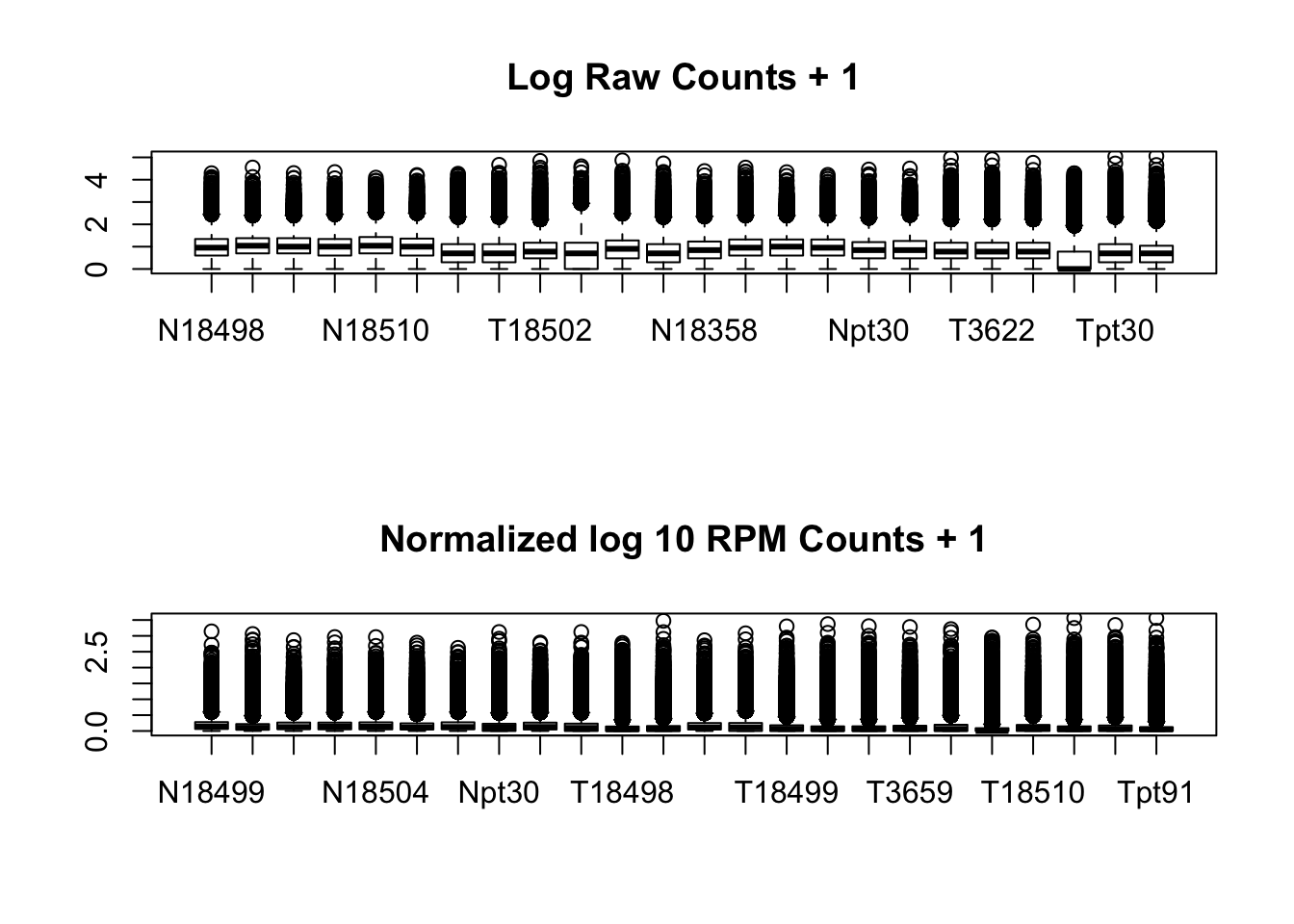
Expand here to see past versions of unnamed-chunk-19-1.png:
| Version | Author | Date |
|---|---|---|
| 6680d6f | brimittleman | 2018-08-27 |
plotDensities(log10(allPeakQuant_matrix_rpm_Norm+1), legend = "bottomright", main="log10 normalized RPM + 1")
abline(v = 0, lty = 3)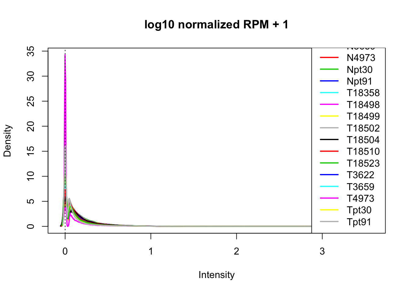
Expand here to see past versions of unnamed-chunk-20-1.png:
| Version | Author | Date |
|---|---|---|
| 6680d6f | brimittleman | 2018-08-27 |
I now have normalized values that are filtered for peaks that had >2 reads.
Differential analysis:
I need to make a design matrix accounting for the two groups each sample can be in. It can be human chimp and total/nuclear. I could also run the analysis seperatly on total and nuclear and just look for differences between hunman and chimp first
Expression matrix:
x=as.matrix(allPeakQuant_matrix_rpm_Norm)Create the feature data- this has 1 row per pas.
f=as.data.frame(rownames(allPeakQuant_matrix_rpm_Norm))
colnames(f)= c("ID")
f = f %>% separate(ID, into=c("Human", "Chimp"), remove = F, sep=":") %>% mutate(name=ID)
f = f %>% column_to_rownames("name")
Create phenotype data frame:
p=read.csv("../data/comp.pheno.data.csv",header = T)
p= p %>% column_to_rownames(var="Sample")
Try a boxplot with these:
boxplot(x[1,]~p[,"Species"], main=f[1,"ID"]) 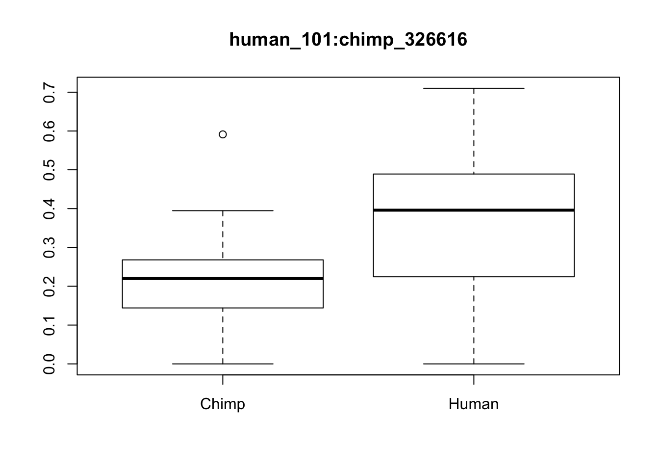
Expand here to see past versions of unnamed-chunk-24-1.png:
| Version | Author | Date |
|---|---|---|
| 2bcaafd | brimittleman | 2018-08-27 |
boxplot(x[1,]~p[,"Fraction"], main=f[1,"ID"]) 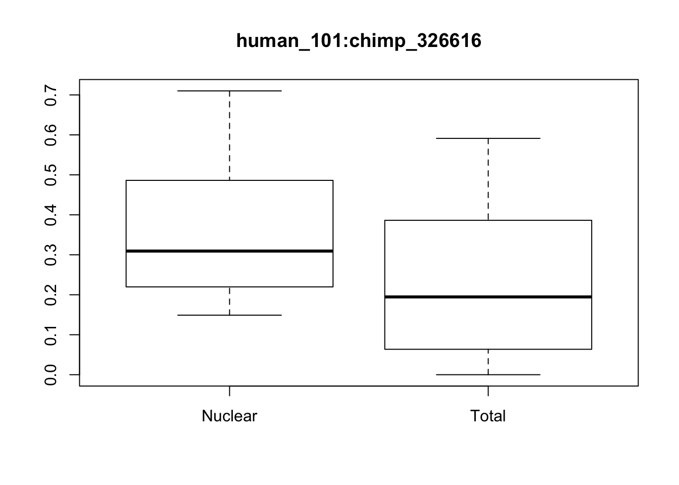
Expand here to see past versions of unnamed-chunk-24-2.png:
| Version | Author | Date |
|---|---|---|
| 2bcaafd | brimittleman | 2018-08-27 |
Create expression set object:
library(Biobase)Loading required package: BiocGenericsLoading required package: parallel
Attaching package: 'BiocGenerics'The following objects are masked from 'package:parallel':
clusterApply, clusterApplyLB, clusterCall, clusterEvalQ,
clusterExport, clusterMap, parApply, parCapply, parLapply,
parLapplyLB, parRapply, parSapply, parSapplyLBThe following object is masked from 'package:limma':
plotMAThe following objects are masked from 'package:dplyr':
combine, intersect, setdiff, unionThe following objects are masked from 'package:stats':
IQR, mad, sd, var, xtabsThe following objects are masked from 'package:base':
anyDuplicated, append, as.data.frame, basename, cbind,
colMeans, colnames, colSums, dirname, do.call, duplicated,
eval, evalq, Filter, Find, get, grep, grepl, intersect,
is.unsorted, lapply, lengths, Map, mapply, match, mget, order,
paste, pmax, pmax.int, pmin, pmin.int, Position, rank, rbind,
Reduce, rowMeans, rownames, rowSums, sapply, setdiff, sort,
table, tapply, union, unique, unsplit, which, which.max,
which.minWelcome to Bioconductor
Vignettes contain introductory material; view with
'browseVignettes()'. To cite Bioconductor, see
'citation("Biobase")', and for packages 'citation("pkgname")'.eset=ExpressionSet(assayData = x,
phenoData = AnnotatedDataFrame(p),
featureData = AnnotatedDataFrame(f))Limma package for DE. Problem, emprical bayes probably relies on independent genes. Some of these peaks go to the same gene, therefore are not indep. I get around this when i use the leafcutter phenotype that is usage of the peak compared to others in the gene. (ill do this later)
First I will do human/chimp as explanatory.
library(limma)
design=model.matrix(~ Species , data=pData(eset))
fit=lmFit(eset,design)
fit=eBayes(fit)
Warning: Zero sample variances detected, have been offset away from zeroresults=decideTests(fit[,"SpeciesHuman"])
summary(results) SpeciesHuman
Down 287
NotSig 75473
Up 447Second I can do this against fraction:
design2=model.matrix(~ Fraction , data=pData(eset))
fit2=lmFit(eset,design2)
fit2=eBayes(fit2)
Warning: Zero sample variances detected, have been offset away from zeroresults2=decideTests(fit2[,"FractionTotal"])
summary(results2) FractionTotal
Down 29626
NotSig 43158
Up 3423Try with both
design3=model.matrix(~ Fraction + Species , data=pData(eset))
fit3=lmFit(eset,design3)
fit3=eBayes(fit3)
Warning: Zero sample variances detected, have been offset away from zeroresults3a=decideTests(fit3[,"FractionTotal"])
results3b=decideTests(fit3[,"SpeciesHuman"])
summary(results3a) FractionTotal
Down 32068
NotSig 40450
Up 3689summary(results3b) SpeciesHuman
Down 924
NotSig 72448
Up 2835It looks like the most peaks are down regulated in total in comparison to nuclear. This makes sense because we expect more peaks to be used in the nuclear fraction.
Session information
sessionInfo()R version 3.5.1 (2018-07-02)
Platform: x86_64-apple-darwin15.6.0 (64-bit)
Running under: macOS Sierra 10.12.6
Matrix products: default
BLAS: /Library/Frameworks/R.framework/Versions/3.5/Resources/lib/libRblas.0.dylib
LAPACK: /Library/Frameworks/R.framework/Versions/3.5/Resources/lib/libRlapack.dylib
locale:
[1] en_US.UTF-8/en_US.UTF-8/en_US.UTF-8/C/en_US.UTF-8/en_US.UTF-8
attached base packages:
[1] parallel stats graphics grDevices utils datasets methods
[8] base
other attached packages:
[1] Biobase_2.40.0 BiocGenerics_0.26.0 edgeR_3.22.3
[4] limma_3.36.3 bindrcpp_0.2.2 cowplot_0.9.3
[7] reshape2_1.4.3 forcats_0.3.0 stringr_1.3.1
[10] dplyr_0.7.6 purrr_0.2.5 readr_1.1.1
[13] tidyr_0.8.1 tibble_1.4.2 ggplot2_3.0.0
[16] tidyverse_1.2.1 workflowr_1.1.1
loaded via a namespace (and not attached):
[1] locfit_1.5-9.1 tidyselect_0.2.4 haven_1.1.2
[4] lattice_0.20-35 colorspace_1.3-2 htmltools_0.3.6
[7] yaml_2.2.0 rlang_0.2.2 R.oo_1.22.0
[10] pillar_1.3.0 glue_1.3.0 withr_2.1.2
[13] R.utils_2.7.0 modelr_0.1.2 readxl_1.1.0
[16] bindr_0.1.1 plyr_1.8.4 munsell_0.5.0
[19] gtable_0.2.0 cellranger_1.1.0 rvest_0.3.2
[22] R.methodsS3_1.7.1 evaluate_0.11 labeling_0.3
[25] knitr_1.20 broom_0.5.0 Rcpp_0.12.18
[28] scales_1.0.0 backports_1.1.2 jsonlite_1.5
[31] hms_0.4.2 digest_0.6.16 stringi_1.2.4
[34] grid_3.5.1 rprojroot_1.3-2 cli_1.0.0
[37] tools_3.5.1 magrittr_1.5 lazyeval_0.2.1
[40] crayon_1.3.4 whisker_0.3-2 pkgconfig_2.0.2
[43] xml2_1.2.0 lubridate_1.7.4 assertthat_0.2.0
[46] rmarkdown_1.10 httr_1.3.1 rstudioapi_0.7
[49] R6_2.2.2 nlme_3.1-137 git2r_0.23.0
[52] compiler_3.5.1 This reproducible R Markdown analysis was created with workflowr 1.1.1