RTG product usage - baseline progressions
This chapter provides baseline task progressions that describe best-practice use of the product for data analysis.
Human read mapping and sequence variant detection
Use the following steps to detect all sequence variants between a reference genome and a sequenced DNA sample or set of related samples. This set of tasks steps through the main functionality of the RTG variant detection software pipeline: generating and evaluating gapped alignments, testing coverage depth, and calling sequence variants (SNPs, MNPs, and indels). While this progression is aimed at human variant detection, the process can easily accommodate other mammalian genomes. For non-mammalian species, some features such as sex and pedigree-aware mapping and variant calling may need to be omitted.
The following example supports the steps typical to human whole exome or whole genome analysis in which high-throughput sequencing with Illumina sequencing systems has generated reads of length 100 to 300 base pairs and at 25 to 30× genome coverage.
RTG features the ability to adjust mapping and variant calling according to the sex of the individual that has been sequenced. During mapping, reads will only be mapped against chromosomes that are present in that individuals genome (for example, for a female individual, reads will not be mapped to the Y chromosome). Similarly, sex-aware variant calling will automatically determine when to switch between diploid and haploid models. In addition, when pedigree information is available, Mendelian inheritance patterns are used to inform the variant calling.
This example demonstrates exome variant calling, automatic sex-aware calling capabilities, and joint variant calling with respect to a pedigree.
Data:
This baseline uses actual data downloaded from public databases. The reference sequence is the human GRCh38, downloaded from ftp://ftp.ncbi.nlm.nih.gov/genomes/all/GCA/000/001/405/GCA_000001405.15_GRCh38/seqs_for_alignment_pipelines.ucsc_ids/GCA_000001405.15_GRCh38_no_alt_plus_hs38d1_analysis_set.fna.gz This version excludes alternate haplotypes but includes the hs38d1 decoy sequence which improves variant calling accuracy by providing targets for reads with high homology to sites on the primary chromosomes.
The read data is from human genome sequencing of the CEPH pedigree 1463, which comprises 17 members across three generations. Illumina sequencing data is provided as part of the Illumina Platinum Genomes project, available via https://www.illumina.com/platinumgenomes.html and also available in the European Nucleotide Archive. Complete Genomics sequencing data for these samples is available via http://www.completegenomics.com/public-data/69-Genomes/
Table : Overview of basic pipeline stages
Task |
Command & Utilities |
Purpose |
|
|---|---|---|---|
1 |
Format reference data |
|
Convert reference sequence from FASTA files to RTG Sequence Data Format (SDF) |
2 |
Prepare pedigree/sex information |
|
Configure per-sample sex and pedigree relationship information in a PED file |
3 |
Format read data |
|
Convert read sequence from FASTA or FASTQ files to RTG Sequence Data Format (SDF) |
4 |
Map reads against a reference genome |
|
Generate read alignments against a given reference, and report in a BAM file for downstream analysis |
5 |
View alignment results |
|
Evaluate alignments and determine if the mapping should be repeated with different settings |
6 |
Generate coverage information |
|
Run the coverage command to generate coverage breadth and depth statistics |
7 |
Call sequence variants (single sample) |
|
Detect SNPs, MNPs, and indels in a sample relative to a reference genome |
8 |
Call sequence variants (single family) |
|
Perform sex-aware joint variant calls relative to the reference on a Mendelian family |
9 |
Call sequence variants (population) |
|
Perform sex-aware joint variant calls relative to the reference on a population |
Task 1 - Format reference data
RTG requires a one-time conversion of the reference genome from FASTA
files into the RTG SDF format. This provides the software with fast
access to arbitrary genomic coordinates in a pre-parsed format. In
addition, metadata detailed autosomes and sex chromosomes is
associated with the SDF, enabling automatic handing of sex chromosomes
in later tasks. This task will be completed with the format
command. The conversion will create an SDF directory containing the
reference genome.
For variant calling and CNV analysis, the reference genome should ideally employ fully assembled chromosomes (as opposed to contig-based coordinates where expected ploidy and inheritance characteristics may be unknown).
First, observe a typical genome reference with multiple chromosomes stored in compressed FASTA format.
$ ls -l /data/human/grch38/fasta
874637925 Feb 28 11:00 GCA_000001405.15_GRCh38_no_alt_plus_hs38d1_analysis_set.fna.gz
Now, use the format command to convert this input file into a single
SDF directory for the reference genome. If the reference is comprised of
multiple input files, these should be supplied on a single command line.
$ rtg format -o grch38 /data/human/grch38/fasta/GCA_000001405.15_GRCh38_no_alt_plus_hs38d1_analysis_set.fna.gz
Formatting FASTA data
Processing "/data/human/grch38/fasta/GCA_000001405.15_GRCh38_no_alt_plus_hs38d1_analysis_set.fna.gz"
Unexpected symbol "M" in sequence "chr1  AC:CM000663.2  gi:568336023  LN:248956422  rl:Chromosome  M5:6aef897c3d6ff0c78aff06ac189178dd  AS:GRCh38" replaced with "N".
[...]

Detected: 'Human GRCh38 with UCSC naming', installing reference.txt

Input Data
Files              : GCA_000001405.15_GRCh38_no_alt_plus_hs38d1_analysis_set.fna.gz
Format             : FASTA
Type               : DNA
Number of sequences: 2580
Total residues     : 3105715063
Minimum length     : 970
Maximum length     : 248956422

Output Data
SDF-ID             : c477b940-e9e7-4068-b7ed-f8968de308e3
Number of sequences: 2580
Total residues     : 3105715063
Minimum length     : 970
Maximum length     : 248956422
This takes the human reference FASTA file and creates a directory called
grch38 containing the SDF. If the reference genome contains IUPAC
ambiguity codes or other non-DNA characters these are replaced with ‘N’
(unknown) in the formatted SDF. The first few such codes will generate
warning messages as above. Every SDF contains a unique SDF-ID
identifier that is reported in log files of subsequent commands and to
help identify potential pipeline issues that arise from incorrectly
using different human reference builds at different pipeline stages.
Note
When formatting a reference genome, the format command
will automatically recognize several common human reference genomes
and install a reference.txt configuration file. For reference
genomes which are not recognized, you should copy or create an
appropriate reference.txt file into the SDF directory if you plan
on performing sex-aware mapping and variant calling. See RTG reference file format
You can use the sdfstats command to show statistics for
your reference SDF, including the individual sequence lengths.
$ rtg sdfstats --lengths grch38
Type               : DNA
Number of sequences: 2580
Maximum length     : 248956422
Minimum length     : 970
Sequence names     : yes
Sex metadata       : yes
Taxonomy metadata  : no
N                  : 165046090
A                  : 868075685
C                  : 599957776
G                  : 602090069
T                  : 870545443
Total residues     : 3105715063
Residue qualities  : no

Sequence lengths:
chr1    248956422
chr2    242193529
chr3    198295559
chr4    190214555
chr5    181538259
chr6    170805979
chr7    159345973
chr8    145138636
chr9    138394717
chr10   133797422
chr11   135086622
chr12   133275309
chr13   114364328
chr14   107043718
chr15   101991189
chr16   90338345
chr17   83257441
chr18   80373285
chr19   58617616
chr20   64444167
chr21   46709983
chr22   50818468
chrX    156040895
chrY    57227415
chrM    16569
chr1_KI270706v1_random  175055
chr1_KI270707v1_random  32032
chr1_KI270708v1_random  127682
[...]
Note the presence of reference chromosome metadata on the line Sex
metadata. This indicates that the information for sex-aware processing
is present. you can use the sdfstats command to verify the
chromosome ploidy information for each sex. For the male sex chromosomes
the PAR region mappings are also displayed.
$ rtg sdfstats grch38 --sex male --sex female
[...]
Sequences for sex=MALE:
chr1 DIPLOID linear 248956422
chr2 DIPLOID linear 242193529
chr3 DIPLOID linear 198295559
chr4 DIPLOID linear 190214555
chr5 DIPLOID linear 181538259
chr6 DIPLOID linear 170805979
chr7 DIPLOID linear 159345973
chr8 DIPLOID linear 145138636
chr9 DIPLOID linear 138394717
chr10 DIPLOID linear 133797422
chr11 DIPLOID linear 135086622
chr12 DIPLOID linear 133275309
chr13 DIPLOID linear 114364328
chr14 DIPLOID linear 107043718
chr15 DIPLOID linear 101991189
chr16 DIPLOID linear 90338345
chr17 DIPLOID linear 83257441
chr18 DIPLOID linear 80373285
chr19 DIPLOID linear 58617616
chr20 DIPLOID linear 64444167
chr21 DIPLOID linear 46709983
chr22 DIPLOID linear 50818468
chrX HAPLOID linear 156040895 ~=chrY
    chrX:10001-2781479  chrY:10001-2781479
    chrX:155701383-156030895  chrY:56887903-57217415
chrY HAPLOID linear 57227415 ~=chrX
    chrX:10001-2781479  chrY:10001-2781479
    chrX:155701383-156030895  chrY:56887903-57217415
chrM POLYPLOID circular 16569
chr1_KI270706v1_random DIPLOID linear 175055
[...]

Sequences for sex=FEMALE:
chr1 DIPLOID linear 248956422
chr2 DIPLOID linear 242193529
chr3 DIPLOID linear 198295559
chr4 DIPLOID linear 190214555
chr5 DIPLOID linear 181538259
chr6 DIPLOID linear 170805979
chr7 DIPLOID linear 159345973
chr8 DIPLOID linear 145138636
chr9 DIPLOID linear 138394717
chr10 DIPLOID linear 133797422
chr11 DIPLOID linear 135086622
chr12 DIPLOID linear 133275309
chr13 DIPLOID linear 114364328
chr14 DIPLOID linear 107043718
chr15 DIPLOID linear 101991189
chr16 DIPLOID linear 90338345
chr17 DIPLOID linear 83257441
chr18 DIPLOID linear 80373285
chr19 DIPLOID linear 58617616
chr20 DIPLOID linear 64444167
chr21 DIPLOID linear 46709983
chr22 DIPLOID linear 50818468
chrX DIPLOID linear 156040895
chrY NONE linear 57227415
chrM POLYPLOID circular 16569
chr1_KI270706v1_random DIPLOID linear 175055
[...]
Task 2 - Prepare sex/pedigree information
RTG commands for mapping and variant calling multiple samples make use of a pedigree file specifying sample names, their sex, and any relations between them. This is done by creating a standard PED format file containing information about the individual samples using a text editor. For example a PED file for the CEPH 1463 pedigree looks like the following.
$ cat population.ped
# PED format pedigree for CEPH/Utah 1463
# fam-id        ind-id  pat-id  mat-id  sex     phen
1       NA12889 0       0       1       0
1       NA12890 0       0       2       0
1       NA12877 NA12889 NA12890 1       0
2       NA12891 0       0       1       0
2       NA12892 0       0       2       0
2       NA12878 NA12891 NA12892 2       0
3       NA12879 NA12877 NA12878 2       0
3       NA12880 NA12877 NA12878 2       0
3       NA12881 NA12877 NA12878 2       0
3       NA12882 NA12877 NA12878 1       0
3       NA12883 NA12877 NA12878 1       0
3       NA12884 NA12877 NA12878 1       0
3       NA12885 NA12877 NA12878 2       0
3       NA12886 NA12877 NA12878 1       0
3       NA12887 NA12877 NA12878 2       0
3       NA12888 NA12877 NA12878 1       0
3       NA12893 NA12877 NA12878 1       0
A value of 0 indicates the field is unknown or that the sample is not
present. Note that the IDs used in columns 2, 3, and 4 must match the
sample IDs used during data formatting and variant calling. The sex
field (column 5) may be 0 if the sex of a sample is unknown. The
family ID in column 1 is ignored as RTG identifies family units
according to the relationship information. You can use the
pedstats command to verify the correct format:
$ rtg pedstats ceph-1463.ped
Pedigree file: ceph-1463.ped
Total samples:               17
Primary samples:             17
Male samples:                 9
Female samples:               8
Afflicted samples:            0
Founder samples:              4
Parent-child relationships:  26
Other relationships:          0
Families:                     3
The pedstats command can also output the pedigree structure in a
format that can be displayed using the dot command from the
Graphviz suite.
$ dot -Tpng <(rtg pedstats --dot "CEPH 1463" ceph-1463.ped) -o ceph-1463.png
This will create a PNG image that can be displayed in any image viewing tool.
$ firefox ceph-1463.png
This will display the pedigree structure as shown below.
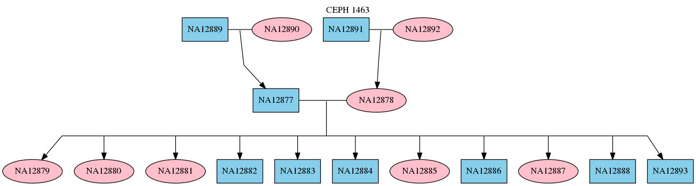
For more information about the PED file format see Pedigree PED input file format.
Task 3 - Format read data
RTG mapping tools accept input read sequence data either in the RTG SDF format or other common sequence formats such as FASTA, FASTQ, or SAM/BAM. There are pros and cons as to whether to perform an initial format of the read sequence data to RTG SDF:
Pre-formatting requires an extra one-off workflow step (the
formatcommand), whereas native input file formats are directly accepted by many RTG commands.Pre-formatting requires extra disk space for the SDF (although these can be deleted after processing if required).
With pre-formatting, decompression, parsing and error checking raw files is carried out only once, whereas native formats require this processing each time.
Pre-formatting permits random access to individual sequences or blocks of sequences, whereas with native formats, the whole file leading up to the region of interest must also be decompressed, and parsed.
Pre-formatting permits loading of sequence data, sequence names, and sequence quality values independently, allowing reduced RAM use during mapping
Thus, pre-formatting read sequence data can result in lower overall resource requirements (and faster throughput) than processing native file formats directly.
In this example we will be converting read sequence data from FASTQ
files into the RTG SDF format. This task will be completed with the
format command. The conversion will create one or more SDF
directories for the reads.
Take a paired set of reads in FASTQ format and convert it into RTG data format (SDF). This example shows one lane of data, taking as input both left and right paired files from the same run.
$ mkdir sample_NA12878
$ rtg format -f fastq -q sanger -o sample_NA12878/NA12878_L001 \
    -l /data/reads/NA12878/NA12878_L001_1.fq.gz \
    -r /data/reads/NA12878/NA12878_L001_2.fq.gz \
    --sam-rg "@RG\\tID:NA12878_L001\\tSM:NA12878\\tPL:ILLUMINA"
This creates a directory named NA12878_L001 with two subdirectories,
named left and right. Use the sdfstats command to verify
this step.
$ rtg sdfstats sample_NA12878/NA12878_L001
It is good practice to ensure the output BAM files contain tracking
information regarding the read set. This is achieved by storing the
tracking information in the reads SDF by using the --sam-rg flag to
provide a SAM-formatted read group header line. The header should
specify at least the ID, SM and PL fields for the read
group. The platform field (PL) values currently recognized by the
RTG command for this attribute are ILLUMINA, LS454,
IONTORRENT, COMPLETE, and COMPLETEGENOMICS. This information
will automatically be used during mapping to enable automatic creation
of calibration files that are used to perform base-quality recalibration
during variant calling. In addition, the sample field (SM) is used
to segregate samples when using multi-sample variant calling commands
such as family, population, and somatic, and should
correspond to the sample ids used in the corresponding pedigree file.
The read group id field (ID) is a
unique identifier used to group of reads that have the same source DNA
and sequencing characteristics (for example, pertain to the same
sequencing lane for the sample). For more details see Using SAM/BAM Read Groups in RTG map.
If the read group information is not specified when formatting the reads,
it can be set during mapping instead using the --sam-rg flag of map.
Repeat this step for all available read data associated with the sample or
samples to be processed. This example shows how this can be done with the
format command in a loop.
$ for left_fq in /data/reads/NA12878/NA12878*_1.fq.gz; do
    right_fq=${left_fq/_1.fq.gz/_2.fq.gz}
    lane_id=$(basename ${left_fq/_1.fq.gz})
    rtg format -f fastq -q sanger -o ${lane_id} -l ${left_fq} -r ${right_fq} \
      --sam-rg "@RG\tID:${lane_id}\tSM:NA12878\tPL:ILLUMINA"
  done
RTG supports the custom read structure of Complete Genomics data. In
this case, use the cg2sdf command to convert the GGI .tsv files into
RTG SDF format. This example shows one run of data, taking as input a
CGI read data file. It is important when mapping Complete Genomics
reads that your read group information should set the platform field
(PL) appropriately. For version 1 reads (35 base-pair reads), the
platform should be COMPLETE. For version 2 reads (29 or 30 base-pair
reads) the platform should be COMPLETEGENOMICS.
$ rtg cg2sdf -o sample_NA12878/NA12878_GS002290 /data/reads/cg/NA12878/GS002290.tsv \
    --sam-rg "@RG\tID:GS002290\tSM:NA12878\tPL:COMPLETE"
As with the formatting of Illumina data, this creates a directory named
GS00290 with two subdirectories, named left and right. You can use
the sdfstats command to verify this step.
$ rtg sdfstats sample_NA12878/NA12878_GS002290
Notice that during formatting we used the same sample identifier for both the Illumina and Complete Genomics data, which allows subsequent variant calling to associate both read sets with the NA12878 individual.
Repeat the formatting for other samples to be processed. When formatting data sets corresponding to other members of the pedigree, be sure to use the correct sample identifier for each individual.
Task 4 - Map reads to the reference genome
Map the sequence reads against the human reference genome to generate alignments in the BAM (Binary Sequence Alignment/Map) file format.
The RTG map command provides multiple tuning parameters to adjust
sensitivity and selectivity at the read mapping stage. In general, whole
genome mapping strategies aim to capture the highest number of reads
possessing variant data and which map with a high degree of specificity
to the human genome. Complete Genomics data has particular mapping
requirements, and for this data use the separate cgmap command.
Depending on the downstream analysis required, the mapping may be adjusted to restrict alignments to unique genomic positions or to allow reporting of ambiguous mappings at equivalent regions throughout the genome. This example will show the recommended steps for human genome analysis.
By default, the mapping will report positions for all mated pairs and unmated reads that map to the reference genome to 5 or fewer positions, those with no good alignments or with more than 5 equally good alignment positions are considered unmapped and are flagged as such in the output.
Note that when mapping each individual we supply the pedigree file with
--pedigree to automatically determine the appropriate sex to be used
when mapping each sample. For a female sample, this will result in no
mappings being made to the Y chromosome. It is also possible to
manually specify the sex of each sample via --sex=male or
--sex=female as appropriate, but using the pedigree file streamlines
the process across all samples.
For the whole-genome Illumina data, a suitable map command is:
$ mkdir map_sample_NA12878
$ rtg map -t grch38 --pedigree ceph-1463.ped \
    -i sample_NA12878/NA12878_L001 -o map_sample_NA12878/NA12878_L001 \
For Complete Genomics reads we use the cgmap command.
$ mkdir cgmap_sample_NA12878
$ rtg cgmap -t grch38 --pedigree ceph-1463.ped --mask cg1 \
    -i sample_NA12878/NA12878_GS002290 -o map_sample_NA12878/NA12878_GS002290 \
The selection of the --mask parameter depends on the length of the
Complete Genomics reads to be mapped. The cg1 and cg1-fast masks are
appropriate for 35 base-pair reads and the cg2 mask is appropriate for
29 or 30 base-pair reads. See cgmap for more
detail.
When the mapping command completes, multiple files will have been
written to the output directory of the mapping run. By default the
alignments.bam file is produced and a BAM index
(alignments.bam.bai) is automatically created to permit efficient
extraction of mappings within particular genomic regions. This
behavior is necessary for subsequent analysis of the mappings, but can
be performed manually using the index command.
During mapping RTG automatically creates a calibration file
(alignments.bam.calibration) containing information about base
qualities, average coverage levels, etc. This calibration information is
utilized during variant calling to improve accuracy and to
determine when coverage levels are abnormally high. When processing
exome or other targeted data, it is important that this calibration
information should only be computed for mappings within the exome
capture regions, otherwise the computed typical coverage levels will be
much lower than actual. This can result in RTG discarding many variant
calls as being over-coverage. The correct workflow for exome
processing is to specify --bed-regions to supply a BED file
describing the exome regions at the same time as mapping, to ensure
appropriate calibration is computed.
$ rtg map -t grch38 --pedigree ceph-1463.ped --bed-regions exome-regions.bed \
    -i sample_NA12878/NA12878_L001 -o map_sample_NA12878/NA12878_L001 \
Note that supplying a BED file does restrict the locations to which reads are mapped, it is only used to ensure calibration information is correctly calculated.
Note
The exome capture BED file must correspond to the correct reference you are mapping and calling against. You may need to run the BED file supplied by your sequencing vendor through a lift-over tool if the reference genome versions differ.
The size of the job should be tuned to the available memory of the
server node. You can perform mapping in segments by using the
--start-read and --end-read flags during mapping. Currently, a
48 GB RAM system as specified in the technical requirements section can
process 100 million reads in about an hour. The following example would work to
map a data set containing just over 100 million reads in batches of 10 million.
$ for ((j=0;j<10;j++)); do
    rtg map -t grch38 --pedigree ceph-1463.ped \
      -i sample1-100M -o map_sample1-$j \
      --start-read=$((j*10000000)) --end-read=$(((j+1)*10000000))
  done
Note that each of these runs can be executed independently of the others. This allows parallel processing in a compute cluster that can reduce wall clock time.
In a parallel compute cluster special consideration is needed with respect to where data resides during the mapping process. Reading and writing data from and to a single networked disk partition may result in undesirable I/O performance characteristics depending on the size and structure of the compute cluster. One way to minimize the adverse affects of I/O limitations is to separate input data sets and map output directories, storing them on different network disk partitions.
Using the --tempdir flag allows the map command to use a
directory other than the output directory to store temporary files that
are output during the mapping process. The size of the temporary files
is the same as the total size of files in the map output directory after
processing has finished. The following example shows how to modify the
above example to place outputs on a separate partition to the inputs.
$ mkdir /partition3/map_temp_sample1
$ for ((j=0;j<10;j++)); do
    rtg map -t /partition1/grch38 --pedigree /partition1/ceph-1463.ped \
      -i /partition1/sample1-100M \
      -o /partition2/map_sample1-$j \
      --start-read=$((j*1000000)) --end-read=$(((j+1)*1000000)) \
      --tempdir /partition3/map_temp_sample1
  done
Processing other samples in the pedigree is a matter of specifying different input SDF and output directories.
Task 5 - View and evaluate mapping performance
An alignments.bam file can be viewed directly using the RTG
extract command in conjunction with a shell command such as less
to quickly inspect the results.
$ rtg extract map_sample_NA12878/NA12878_L001-0/alignments.bam | less -S
Since the mappings are indexed by default, it is also possible to view mappings corresponding to particular genomic regions. For example:
$ rtg extract map_sample_NA12878/NA12878_L001-0/alignments.bam chr6:1000000-5000000 \
  | less -S
The mapping output directory also contains a simple HTML summary report giving information about mapping counts, alignment score distribution, paired-end insert size distribution, etc. This can be viewed in your web browser. For example:
$ firefox map_sample_NA12878/NA12878_L001-0/index.html
For more detailed summary statistics, use the samstats command. This
example will report information such as total records, number unmapped,
specific details about the mate pair reads, and distributions for
alignment scores, insert sizes and read hits.
$ rtg samstats -t grch38 map_sample_NA12878/NA12878_L001-0/alignments.bam \
   -r sample_NA12878/NA12878_L001 --distributions
Finally, the short summary of mapping produced on the terminal at the end of
the map run, is also available as summary.txt in the mapping output
directory.
Task 6 - Generate and review coverage information
For human genomic analysis, it is important to have sufficient coverage
over the entire genome to detect variants accurately and minimize false
negative calls. The coverage command provides detailed statistics for
depth of coverage and gap size distribution. If coverage proves to be
inadequate or spotty, remapping the data with different sensitivity tuning
or rerunning the sample with different sequencing technology may help.
This example shows the coverage command used with all alignments, both
mated and unmated, for the entire sample. The -s flag is used to
introduce smoothing of the data, by default the data will not be
smoothed. While you can supply the coverage command with the names of
BAM files individually on the command line, this becomes unwieldy when
the mapping has been carried out in many smaller jobs. In this command
we will use the -I flag to supply a text file containing the names of
all the mapping output BAM files, one per line. One example way to
create this file is with the following command (assuming all your
mapping runs have used a common root directory):
$ find map_sample_NA12878 -name "*.bam" > NA12878-bam-files.txt
$ rtg coverage -t grch38 -s 20 -o cov_sample_NA12878 -I NA12878-bam-files.txt
For exome or other targeted data, the coverage command can be instructed to focus only within the target regions by supplying the target regions BED file.
$ rtg coverage -t grch38 --bed-regions exome-regions.bed -s 20 \
    -o cov_sample_NA12878 -I NA12878-bam-files.txt
By default the coverage command will generate a BED formatted file
containing regions of similar coverage. This BED file can be loaded into
a genome browser to visualize the coverage, and may also be examined on
the command line. For example:
$ rtg extract cov_sample_NA12878/coverage.bed.gz 'chr6:1000000-5000000' | less
The coverage command also creates a simple HTML summary report
containing graphs of the depth of coverage distribution and cumulative
depth of coverage. This can be viewed in your web browser. For example:
$ firefox cov_sample_NA12878/index.html
The coverage command has several options that alter the way that
coverage levels are reported (for example, determining callability or
giving per-region reporting). See coverage for more detail.
Task 7 - Call sequence variants (single sample)
The primary germline variant calling commands in the RTG suite are the
snp command for detecting variants in a single sample, the
family command for performing simultaneous joint calling of multiple
family members within a single family, and the population command
for performing simultaneous joint calling of multiple population members
with varying degrees of relatedness. Where possible, we recommend using
joint calling, as this ensures the maximum use of pedigree information
as well as preventing cross-sample variant representation inconsistency
that can occur when calling multiple samples individually. All of the
RTG variant callers are sex-aware, producing calls of appropriate ploidy
on the sex chromosomes and within PAR regions.
In this section, we demonstrate single sample calling with snp. For
family calling, see Task 8 - Call sequence variants (single family), and for population calling,
see Task 9 - Call population sequence variants.
The snp command detects sequence variants in a single sample, given
adequate but not excessively high coverage of reads against the
reference genome. As with the coverage command, we can supply a file
containing a list of all the needed input files. In this case the
mapping calibration files will be automatically detected at the location
of the BAM files themselves and will be used in order to enable base
quality recalibration during variant calling.
This example takes all available BAM files for the sample and calls SNP, MNP, and indel sequence variants.
$ rtg snp -t grch38 --pedigree ceph-1463.ped \
    -o snp_sample_NA12878 -I sample_NA12878-bam-files
Here we supply the pedigree file in order to inform the variant caller
of the sample sex. While multiple samples may be listed in the pedigree
file, the snp command will object if mappings for multiple samples
are supplied as input.
For exome data it is also recommended to provide the BED file describing
the exome regions to the variant caller in order to filter the output
produced to be within the exome regions. There are two approaches
here. The first is to instruct the variant caller to only perform
variant calling at sites within the exome regions by supplying the
--bed-regions option:
$ rtg snp -t grch38 --pedigree ceph-1463.ped -–bed-regions exome-regions.bed \
    -o snp_sample_NA12878 -I sample_NA12878-bam-files
This approach is computationally more efficient. However, if calls at
off-target sites are potentially of interest, a second approach is to
call variants at all sites but automatically filter variants as being
off-target in the VCF FILTER field by using the --filter-bed option:
$ rtg snp -t grch38 --pedigree ceph-1463.ped --filter-bed exome-regions.bed \
    -o snp_sample_NA12878 -I sample_NA12878-bam-files
If you do not have a BED file that specifies the exome capture regions
for your reference genome, you should supply the --max-coverage flag
during variant calling to indicate an appropriate coverage threshold for
over-coverage situations. A typical value is 5 times the expected
coverage level within exome regions.
The snp command will perform the Bayesian variant calling and will
use a default AVR model for scoring variant call quality. If you have a
more appropriate model available, you should supply this with the
--avr-model flag. RTG supplies some pre-built models which work well
in a wide variety of cases, and includes tools for building custom AVR
models. See AVR scoring using HAPMAP for model building for more
information on building custom models.
The snp command will output variant call summary information upon
completion, and this is also available in the output directory in the
file summary.txt.
Variants are produced in standard VCF format. Since the variant calls are compressed and indexed by default, it is possible to view calls corresponding to particular genomic regions. For example:
$ rtg extract snp_sample_NA12878/snps.vcf.gz chr6:1000000-5000000 | less -S
Inspecting the output VCF for this run will show that no variants have been called for the Y chromosome. If you carry out similar sex-aware calling for the father of the trio, NA12891, inspection of the output VCF will show haploid variant calls for the X and Y chromosomes.
$ rtg extract snp_sample_NA12891/snps.vcf.gz chrX | head
$ rtg extract snp_sample_NA12891/snps.vcf.gz chrY | head
RTG also supports automatic handling of pseudoautosomal regions (PAR) and will produce haploid or diploid calls within the X PAR regions as appropriate for the sex of the individual.
A simple way to improve throughput is to call variants using a separate job for each reference sequence. Each of these runs could be executed on independent nodes of a cluster in order to reduce wall clock time.
$ for seq in M {1..22} X Y; do
    rtg snp -t grch38 --pedigree ceph-1463.ped -I sample_NA12878-bam-files \
      -o snp_sample_NA12878_chr"$seq" --region chr"$seq"
  done
After the separate variant calling jobs complete, the VCF files for each
chromosome can be combined into a single file, if desired, by using a
vcfmerge command such as:
$ rtg vcfmerge -o snp_sample_NA12878.vcf.gz snp_sample_NA12878_chr*/snps.vcf.gz
The individual snp commands will have output summary information about
the variant calls made in each job. Combined summary information can be
output for the merged VCF file with the vcfstats command.
$ rtg vcfstats snp_sample_NA12878.vcf.gz
Simple filtering of variants can be applied using the vcffilter
command. For example, filtering calls by genotype quality or AVR score
can be accomplished with a command such as:
$ rtg vcffilter --min-genotype-quality 50 -i snp_sample_NA12878.vcf.gz \
  -o filtered_sample_NA12878.vcf.gz
In this case, any variants failing the filter will be removed.
Alternatively, failing variants can be kept but marked with a custom VCF
FILTER field, such as:
$ rtg vcffilter --fail LOW-GQ --min-genotype-quality 50 \
  -i snp_sample_NA12878.vcf.gz -o filtered_sample_NA12878.vcf.gz
Task 8 - Call sequence variants (single family)
This section demonstrates joint calling multiple samples comprising a single Mendelian family. RTG is unique in supporting family calling beyond a single-child trio, and directly supports jointly calling a family involving multiple offspring. In this example, we call the large family of the CEPH pedigree containing 11 children.
The family command is invoked similarly to the snp command except
you need to specify the way the samples relate to each other. This is
done by specifying the corresponding sample ID used during mapping to the
command line flags --mother, --father, --daughter and --son.
Note
The RTG family command only supports a basic
family relationship of a mother, father and one or more children, either
daughters or sons. For other pedigrees, use the population command.
To run the family command on the trio of NA12892 (mother), NA12891
(father) and NA12878 (daughter) you need to provide all the mapping
files for the samples. The mapping calibration files will be
automatically detected at the locations of the mapping files. To specify
these in a file list for input you could run:
$ find /partition2/map_trio -name "alignments.bam" > map_trio-bam-files
To run the family command you then specify the sample ID for each member
of the trio to the appropriate flag.
$ rtg family --mother NA12892 --father NA12891 --daughter NA12878 -t grch38 \
  -o trio_variants -I map_trio-bam-files
Examining the snps.vcf.gz file in the output directory will show
individual columns for the variants of each family member. For more
details about the VCF output file see Small-variant VCF output file description
Note
Per-family relationship information can also be specified
using a pedigree PED file with the --pedigree flag. In this case,
the pedigree file should contain a single family only.
Task 9 - Call population sequence variants
This section demonstrates joint variant calling of multiple potentially related or unrelated individuals in a population.
The population command is invoked similarly to the snp command
except you must specify the pedigree file containing information about
each sample and the relationships (if any) between them.
To run the population command on the population of NA12892, NA12891,
NA19240 and NA12878 you need to provide all the mapping files for the
samples. The mapping calibration files will be automatically detected at
the locations of the mapping files. To specify these in a file list for
input you could run:
$ find /partition2/map_population -name "alignments.bam" > map_population-bam-files
To run the population command you specify the PED file containing
the sample ID for each member of the population in the individual ID
column.
$ rtg population -t grch38 --pedigree ceph-1463.ped -o pop_variants \
    -I map_population-bam-files
Examining the snps.vcf.gz file in the output directory will show
individual columns for the variants of each member of the population.
For more details about the VCF output file see
Small-variant VCF output file description.
Create and use population priors in variant calling
To improve the accuracy of variant calling on new members of a population, a file containing the allele counts of the population’s known variants may be supplied. This information is used as an extra set of prior probabilities when making calls.
Sources of this allele count data can be external, for instance the 1000 genomes project, or from prior variant calling on other members of the population. An example use case of the latter follows.
Data
For this use case it is assumed that the following data is available:
/data/runs/20humans.vcf.gz- output from a previous population command run on 20 humans from a population./data/reference/human_reference- SDF containing the human reference sequences./data/mappings/new_human.txt- text file containing a list of BAM files with the sequence alignments for the new member of the population.
Table : Overview of pipeline tasks.
Task |
Command & Utilities |
Purpose |
|
|---|---|---|---|
1 |
Produce population priors file |
|
Produce a reusable set of population priors from an existing VCF file |
2 |
Run variant calling using population priors |
|
Perform variant calling on the new member of the population using the new population priors to improve results |
Task 1 - Produce population priors file
Using a full VCF file for a large population as population priors can be
slow, as it contains lots of unnecessary information. The AC and AN
fields are the standard VCF specification fields representing the allele
count in genotypes, and total number of alleles in called genotypes. For
more information on these fields, see the VCF specification at
https://samtools.github.io/hts-specs/VCFv4.2.pdf. Alternatively,
retaining only the GT field for each sample is sufficient, however
this is less efficient both computationally and size-wise.
To calculate and annotate the AC and AN fields for a VCF file, use
the RTG command vcfannotate with the parameter --fill-an-ac:
$ rtg vcfannotate --fill-an-ac -i /data/runs/20humans.vcf.gz \
  -o 20humans_an_ac.vcf.gz
Then remove all unnecessary data from the file using the RTG command
vcfsubset as follows:
$ rtg vcfsubset --keep-info AC,AN --remove-samples \
  -i 20humans_an_ac.vcf.gz -o 20humans_priors.vcf.gz
This output is block compressed and tabix indexed by default, which is
necessary for the population priors input. There will be an additional
file output called 20humans_priors.vcf.gz.tbi which is the tabix
index file.
The resulting population priors can now be stored in a suitable location to be used for any further runs as required.
$ cp 20humans_priors.vcf.gz* /data/population_priors/
Task 2 - Run variant calling using population priors
The population priors can now be used to improve variant calling on new
members of the population supplying the --population-priors parameter
to any of the variant caller commands.
$ rtg snp -o new_human_snps -t /data/reference/human_reference \
  -I /data/mappings/new_human.txt \
  --population-priors /data/population_priors/20humans_priors.vcf.gz
Somatic variant detection in cancer
RTG includes two variant calling commands for detecting somatic
variations in tumor samples: somatic should be used when data from a
matched normal sample is available; and tumoronly should be used when
there is no matched normal sample.
Follow the steps below to obtain somatic variant calls.
Table : Overview of somatic pipeline tasks.
Task |
Command & Utilities |
Purpose |
|
|---|---|---|---|
1 |
Format reference data |
|
Convert reference sequence from FASTA file to RTG Sequence Data Format (SDF) |
2 |
Format read data |
|
Convert read sequence from FASTA and FASTQ files to RTG Sequence Data Format (SDF) |
3 |
Map reads against the reference genome |
|
Generate read alignments for the sample(s), and report in a BAM file for downstream analysis |
4 |
Call somatic variants |
|
Detect somatic variants in the tumor sample |
Task 1 - Format reference data (Somatic)
Format the human reference data to RTG SDF using Task 1 of RTG mapping
and sequence variant detection. In the following tasks it is assumed
the human reference SDF is called grch38.
Task 2 - Format read data (Somatic)
Format the tumor sample read data to RTG SDF using Task 2 of RTG mapping and sequence variant detection. In this example we assume there are 20 lanes of data for the sample.
$ for ((i=1;i<20;i++)); do
$   rtg format -f fastq -q sanger -o tumor_reads_${i} \
    -l /data/reads/tumor/${i}/reads_1.fq \
    -r /data/reads/tumor/${i}/reads_2.fq \
    --sam-rg "@RG\tID:tumor_${lane_id}\tSM:sm_tumor\tPL:ILLUMINA"
  done
When matched normal sample data is available, format this in a similar manner. Note that a different sample name should be supplied for the read group information for the normal sample.
$ for ((i=1;i<20;i++)); do
$   rtg format -f fastq -q sanger -o normal_reads_${i} \
    -l /data/reads/normal/${i}/reads_1.fq \
    -r /data/reads/normal/${i}/reads_2.fq \
    --sam-rg "@RG\tID:normal_${lane_id}\tSM:sm_normal\tPL:ILLUMINA"
  done
Task 3 - Map tumor and normal sample reads against the reference genome
Map the normal and tumor sample reads against the reference genome as in
Task 4 - Map reads to the reference genome. The mapping must be
done with appropriate read group information for each read set, by using
the --sam-rg flag at mapping time unless this has been done during
the format command as described above. All mappings on the tumor should
have one sample ID, and (when available) all mappings on the matched
normal should have another sample ID.
$ for ((i=1;i<20;i++)); do
    rtg map -i tumor_reads_${i} -t grch38 -o tumor_map_${i}
  done
$ for ((i=1;i<20;i++)); do
    rtg map -i normal_reads_${i} -t grch38 -o normal_map_${i}
  done
Task 4 - Call somatic variants
When no matched normal data is available, the tumoronly command is
invoked, similarly to the snp comment. You may optionally specify
an estimated level of contamination of the tumor sample with normal
tissue using the --contamination flag.
$ rtg tumoronly -t grch38 -o tumoronly_out --contamination 0.3 \
  tumor_map_*/alignments.bam
Where a matched normal sample is available, the somatic command is
invoked. Command options are similar to tumoronly, except you need
to specify the sample IDs corresponding to the normal and cancer
samples, with the --original and --derived flags respectively.
- $ rtg somatic -t grch38 -o somatic_out –contamination 0.3
–derived sm_tumor –original sm_normal normal_map_*/alignments.bam tumor_map_*/alignments.bam
Examining the snps.vcf.gz file in the output directory will show a
column each for the variants of the normal and tumor samples and will
contain variants where the tumor sample differs from the normal sample.
The somatic command stores information in the VCF INFO fields NCS,
and LOH, and FORMAT fields SSC and SS. For more details
about the VCF output file see Small-variant VCF output file description.
The somatic command also supports --include-germline to include
variants that are predicted to be germline, in addition to those
predicted to be of somatic origin, in the output VCF.
Using site-specific somatic priors
The tumoronly and somatic commands have a default prior of
0.000001 (1e-6) for a particular site being somatic. Since the human
genome comprises some 3.2 GB, this prior corresponds to an expectation
of about 3200 somatic variants in a whole genome sample. Depending on
the expected number of variants for a particular sample, it may be
appropriate to raise or lower this prior. In general, decreasing the
prior increases specificity while increasing the prior increases
sensitivity.
Of course, not every site is equally likely to lead to a somatic
variant. To support different priors for different sites we provide a
facility to set a prior on per site basis via a BED file we call
site-specific somatic priors. The --somatic-priors command line
option is used to provide the file to the variant caller.
The site-specific somatic priors can cover as many or as few sites as desired. Any site not covered by a specific prior will use the default prior. The format of the file is a BED file where the fourth column of each line gives the explicit prior for the indicated region, for example,
1 14906 14910 1e-8
denotes that the prior for bases 14907, 14908, 14909, and 14910 on chromosome 1 is 1e-8 rather than the default. (Recall that BED files use 0-based indices.) If the BED file contains more than one prior covering a particular site, then the largest prior covering that site is used. When making a complex call, the prior used is the arithmetic average of priors in the region of the complex call.
A typical starting point for making somatic site-specific priors might include a database of known cancer sites (for example, COSMIC) and a database of sites known to be variant in the population (for example, dbSNP). The idea is that the COSMIC sites are more likely to be somatic and should have a higher prior, while those in dbSNP are less likely to be somatic and should have a lower prior.
The following recipe can be used to build the BED file where some sites have a lower prior of 1e-8 and others have a higher prior of 1e-5. The procedure can be easily modified to incorporate additional inputs each with its own prior.
First, collect prerequisites in the form of VCF files (here using the
names cosmic.vcf.gz and dbsnp.vcf.gz, but, of course, any other VCFs
can also be used).
$ COSMIC=cosmic.vcf.gz
$ DBSNP=dbsnp.vcf.gz
Convert each VCF file into a BED file with the desired priors taking care to convert from 1-based coordinates in VCF to 0-based coordinates in VCF.
$ zcat ${COSMIC} | awk -vOFS='\t' '/^[^#]/{print $1,$2-1,$2+length($4)-1,"1e-5"}'\
  | sort -Vu >p0.bed
$ zcat ${DBSNP} | awk -vOFS='\t' '/^[^#]/{print $1,$2-1,$2+length($4)-1,"1e-8"}'\
  | sort -Vu >p1.bed
[Optional] Collapse adjacent intervals together. One way of doing this
is to use the bedtools merge facility. This can result in a smaller
final result when the intervals are dense.
$ bedtools merge -c 4 -o distinct -i p0.bed >p0.tmp && mv p0.tmp p0.bed
$ bedtools merge -c 4 -o distinct -i p1.bed >p1.tmp && mv p1.tmp p1.bed
In general, care must be taken to ensure intersecting sites are handled in the desired manner. Since in this case we want to use COSMIC in preference to dbSNP and prior(COSMIC) > prior(dbSNP), we can simply merge the outputs because the somatic caller will choose the larger prior in the case of overlap.
$ sort --merge -V p0.bed p1.bed | rtg bgzip - >somatic-priors.bed.gz
To support somatic calling on restricted regions, construct a tabix index for the priors file.
$ rtg index -f bed somatic-priors.bed.gz
The site-specific somatic BED file is now ready to be used by the
tumoronly and somatic commands:
$ rtg somatic -–somatic-priors somatic-priors.bed.gz ...
AVR scoring using HAPMAP for model building
AVR (Adaptive Variant Rescoring) is a machine learning technology for learning and predicting which calls are likely correct. It comprises of a learning algorithm that takes training examples and infers a model about what constitutes a good call and a prediction engine which applies the model to variants and estimates their correctness. It includes attributes of the call that are not considered by the internal Bayesian statistics model to make better predictions as to the correctness of a variant call.
Each of the RTG variant callers (snp, family, population)
automatically runs a default AVR model, producing an AVR attribute for
each sample. The model can be changed with the --avr-model parameter,
and the AVR functionality can be turned off completely by specifying the
special ‘none’ model.
Example command line usage. Turn AVR rescoring off:
$ rtg family --mother NA12892 --father NA12891 --daughter NA12878 -t grch38 \
  -o trio_variants -I map_trio-bam-files --avr-model none
Apply default RTG AVR model:
$ rtg family --mother NA12892 --father NA12891 --daughter NA12878 -t grch38 \
  -o trio_variants -I map_trio-bam-files
Apply a custom AVR model:
$ rtg family --mother NA12892 --father NA12891 --daughter NA12878 -t grch38 \
  -o trio_variants -I map_trio-bam-files --avr-model /path/to/my/custom.avr
The effectiveness of AVR is strongly dependent on the quality of the training data. In general, the more training data you have, the better the model will be. Ideally the training data should have the same characteristics as the calls to be predicted; that is, the same platform, the same reference, the same coverage, etc. There also needs to be a balance of positive and negative training examples. In reality, these conditions can only be met to varying degrees, but AVR will try to make the most of what it is given.
A given AVR model is tied to a set of attributes corresponding to fields in VCF records or quantities that are derivable from those fields. The attributes chosen can take into account anomalies associated with different sequencing technologies. Examples of attributes are things like quality of the call, zygosity of the call, strand bias, allele balance, and whether or not the call is complex. Not all attributes are equally predictive and it is the job of the machine learning to determine which combinations of attributes lead to the best predictions. When building a model it is necessary to provide the list of attributes to be used. In general, providing more attributes gives the AVR model a better chance at learning what constitutes a good call. There are two caveats; the attributes used during training need to be present in the calls to be predicted and some attributes like DP are vulnerable to changes in coverage. AVR is able to cope with missing values during both training and prediction.
The training data needs to comprise both positive and negative examples. Ideally we would know exactly the truth status of each training example, but in reality this must be approximated by reference to some combination of baseline information.
In the example that follows, the HAPMAP database will be used to produce and then use an AVR model on a set of output variants, a process that can be used when no appropriate AVR model is already available. The HAPMAP database will be used to determine which of the variants will be considered correct for training purposes. This will introduce two types of error; correct calls which are not in HAPMAP will be marked as negative training examples and a few incorrect calls occurring at HAPMAP sites will be marked as positive training examples.
Data
Reference SDF on which variant calling was performed, in this example assumed to be an existing SDF containing the 1000 genomes build 37 phase 2 reference
(ftp://ftp.1000genomes.ebi.ac.uk/vol1/ftp/technical/reference/phase2_reference_assembly_sequence/hs37d5.fa.gz).
For this example this will be called
/data/reference/1000g_v37_phase2.
The HAPMAP variants file from the Broad Institute data bundle
(ftp://gsapubftp-anonymous@ftp.broadinstitute.org/bundle/2.5/b37/hapmap_3.3.b37.vcf.gz).
For this example this will be called /data/hapmap_3.3.b37.vcf.gz.
The example will be performed on the merged results of the RTG family
command for the 1000 genomes CEU trio NA12878, NA12891 and NA12892. For
this example this will be called /data/runs/NA12878trio/family.vcf.gz.
Table : Overview of basic pipeline tasks.
Task |
Command & Utilities |
Purpose |
|
|---|---|---|---|
1 |
Create training data |
|
To generate positive and negative examples for the AVR machine learning model to train on |
2 |
Build and check AVR model |
|
To create and check an AVR model |
3 |
Use AVR model |
|
To apply the AVR model to the existing output or to use it directly during variant calling |
4 |
Install AVR model |
|
Install model in standard RTG model location for later reuse |
Task 1 - Create training data
The first step is to use the vcffilter command to split the variant
calls into positive and negative training examples with respect to
HAPMAP. It is also possible to build training sets using the vcfeval
command, however this is less appropriate for dealing with sites rather
than calls, and experiments indicate using vcffilter leads to better
training sets.
$ rtg vcffilter --include-vcf /data/hapmap_3.3.b37.vcf.gz -o pos-NA12878.vcf.gz \
  -i /data/runs/NA12878trio/family.vcf.gz --sample NA12878 --remove-same-as-ref
$ rtg vcffilter --exclude-vcf /data/hapmap_3.3.b37.vcf.gz -o neg-NA12878.vcf.gz \
  -i /data/runs/NA12878trio/family.vcf.gz --sample NA12878 --remove-same-as-ref
Optionally check that the training data looks reasonable. There should be a reasonable amount of both positive and negative examples and all expected chromosomes should be represented.
Task 2 - Build and check AVR model
The next step is to build an AVR model. Select the attributes that will
be used with some consideration to portability and the nature of the
training set. Here we have excluded XRX and LAL because HAPMAP is
primarily SNP locations and does not capture complex calls. By excluding
XRX and LAL we prevent the model from learning that complex calls
are bad. We have also excluded DP because we want a model somewhat
independent of coverage level. Building the model can take a large
amount of RAM and several hours. The amount of memory required is
proportional to the number of training instances.
A list of derived annotations that can be used are available in the
documentation for avrbuild. For VCF INFO and FORMAT
annotations check the header of the VCF file for available fields. The
VCF fields output by RTG variant callers are described in Small-variant VCF output file description.
$ rtg avrbuild -o NA12878model.avr --info-annotations DPR \
  --format-annotations DPR,AR,ABP,SBP,RPB,GQ \
  --derived-annotations IC,EP,QD,AN,PD,GQD,ZY \
  --sample NA12878 -p pos-NA12878.vcf.gz -n neg-NA12878.vcf.gz
Examine the statistics output to the screen to check things look reasonable. Due to how attributes are computed there can be missing values, but it is a bad sign if any attribute is missing from most samples.
Total number of examples: 5073752
Total number of positive examples: 680677
Total number of negative examples: 4393075
Total weight of positive examples: 2536873.27
Total weight of negative examples: 2536876.42
Number of examples with missing values:
DERIVED-AN 0
DERIVED-EP 0
DERIVED-GQD 0
DERIVED-IC 915424
DERIVED-PD 0
DERIVED-QD 0
DERIVED-ZY 0
FORMAT-ABP 13602
FORMAT-AR 8375
FORMAT-DPR 0
FORMAT-GQ 0
FORMAT-RPB 8375
FORMAT-SBP 37129
INFO-DPR 0
Hold-out score: 69.1821% (96853407/139997752)
Attribute importance estimate for DERIVED-AN: 0.0304% (29443/96853407)
Attribute importance estimate for DERIVED-EP: 1.2691% (1229135/96853407)
Attribute importance estimate for DERIVED-GQD: 4.7844%
(4633873/96853407)
Attribute importance estimate for DERIVED-IC: 4.7748% (4624554/96853407)
Attribute importance estimate for DERIVED-PD: 0.0000% (0/96853407)
Attribute importance estimate for DERIVED-QD: 6.8396% (6624383/96853407)
Attribute importance estimate for DERIVED-ZY: 0.8693% (841925/96853407)
Attribute importance estimate for FORMAT-ABP: 5.4232% (5252533/96853407)
Attribute importance estimate for FORMAT-AR: 2.6008% (2518955/96853407)
Attribute importance estimate for FORMAT-DPR: 3.3186% (3214163/96853407)
Attribute importance estimate for FORMAT-GQ: 3.4268% (3319009/96853407)
Attribute importance estimate for FORMAT-RPB: 0.2176% (210761/96853407)
Attribute importance estimate for FORMAT-SBP: 0.0219% (21196/96853407)
Attribute importance estimate for INFO-DPR: 4.6525% (4506074/96853407)
Optionally check the resulting model file using the avrstats command.
This will produce a short summary of the model including the attributes
used during the build.
$ rtg avrstats NA12878model.avr
Location : NA12878model.avr
Parameters : avrbuild -o NA12878model.avr --info-annotations DPR --derived-annotations IC,EP,QD,AN,PD,GQD,ZY --format-annotations DPR,AR,ABP,SBP,RPB,GQ --sample NA12878 -p pos-NA12878.vcf.gz -n neg-NA12878.vcf.gz
Date built : 2013-05-17-09-41-17
AVR Version : 1
AVR-ID : 7ded37d7-817f-467b-a7da-73e374719c7f
Type : ML
QUAL used : false
INFO fields : DPR
FORMAT fields : DPR,AR,ABP,SBP,RPB,GQ
Derived fields: IC,EP,QD,AN,PD,GQD,ZY
Task 3 - Use AVR model
The model is now ready to be used. It can be applied to the existing
variant calling output by using the avrpredict command.
$ rtg avrpredict --avr-model NA12878model.avr \
  -i /data/runs/NA12878trio/family.vcf.gz -o predict.vcf.gz
This will create or update the AVR FORMAT field in the VCF output
file with a score between 0 and 1. The higher the resulting score the
more likely it is correct. To select an appropriate cutoff value for
further analysis of variants some approaches might include measuring the
Ti/Tv ratio or measuring sensitivity against another standard such as
OMNI at varying score cutoffs.
The model can also be used directly in any new variant calling runs:
$ rtg snp --avr-model NA12878model.avr -t grch38 -o snp_sample_NA12878 --sex female \
  -I sample_NA12878-map-files
$ rtg population --avr-model NA12878model.avr -t grch38 -o pop_variants \
  -I map_population-bam-files
Task 4 - Install AVR model
The custom AVR model can be installed into a standard location so that
it can be referred to by a short name (rather than the full file path
name) in the avrpredict and variant caller commands. The default
location for AVR models is within a subdirectory of the RTG installation
directory called models, and each file in that directory with a .avr
extension is a model that can be accessed by its short name. For example
if the NA12878model.avr model file is placed in
/path/to/rtg/installation/models/NA12878model.avr it can be accessed
by any user either using the full path to the model:
$ rtg snp --avr-model /path/to/rtg/installation/models/NA12878model.avr \
  -o snp_sample_NA12878 -t grch38 --sex female -I sample_NA12878-map-files
or, by just the model file name:
$ rtg snp --avr-model NA12878model.avr -o snp_sample_NA12878 -t grch38 --sex female \
  -I sample_NA12878-map-files
The AVR model directory will already contain the models prebuilt by RTG:
illumina-exome.avr- model built from Illumina exome sequencing data. If you are running variant calling Illumina exome data you may want to use this model instead of the default, although the default should still be effective.illumina-wgs.avr- model built from Illumina whole genome sequencing data. This model is the default model when running normal variant calling.illumina-somatic.avr- model built from somatic samples usingIllumina sequencing. It is applicable to somatic variant calling, where a variety of allelic fractions are to be expected in somatic variants. The
somaticcommand defaults to this AVR model. If you want to score germline variants in a somatic run, it is preferable to useillumina-wgs.avrorillumina-exome.wgsinstead.
alternate.avr- model built usingXRX,ZYandGQDattributes. This should be platform independent and may be a better choice if a more specific model for your data is unavailable. In particular, this model may be more appropriate for scoring the results of variant calling in situations where unusual allele-balance is expected (for example somatic calling with contamination, or calling high amplification data where allele drop out is expected)
It is possible to score a sample with more than one AVR model, by running
avrpredict with another model and using a different field name
specified with --vcf-score-field.
RTG structural variant detection
RTG has developed tools to assist in discovering structural variant regions in whole genome sequencing data. The tools can be used to locate likely structural variant breakpoints and regions that have been duplicated or deleted. These tools are capable of processing whole genome mapping data containing multiple read groups in a streamlined fashion.
In this example, it is assumed that alignment has been carried out as
described in Task 4 - Map reads to the reference genome. For
structural variant detection it is particularly important to specify the
read group information with the --sam-rg flag either during the
formatting of the reads or for the map command explicitly. The
structural variant tools currently requires the PL (platform)
attribute to be either ILLUMINA (for Illumina reads) or COMPLETE
(for Complete Genomics reads).
Table : Overview of structural variants analysis pipeline tasks.
Task |
Command & Utilities |
Purpose |
|
|---|---|---|---|
1 |
Prepare read group statistics file |
|
Identify read group statistics files created during mapping |
2 |
Find structural variants with sv |
|
Process prepared mapping results to identify likely structural variants |
3 |
Find structural variants with discord |
|
Process prepared mapping results to identify likely structural variant breakends |
4 |
Find copy number variants |
|
Detect copy number variants between a pair of samples |
Task 1 - Prepare Read-group statistics files
Mapping identifies discordant read matings and inserts the pair
information for unique unmated reads into the SAM records. The map
command also produces a file within the directory called rgstats.tsv
containing read group statistics.
The sv and discord structural variant callers require the read
group statistics files to be supplied, so as with multiple BAM files, it
is possible to create a text file listing the locations of all the
required statistics files:
$ find /partition2/map_sample_NA12878 -name "rgstats.tsv" \
  > sample_NA12878-rgstats-files
Task 2 - Find structural variants with sv
Once mapping is complete one can run the structural variants analysis
tool. To run the sv tool you need to supply the mapping BAM files
and the read group statistics files. As with the variant caller
commands, this can be a large number of files and so input can be
specified using list files.
$ rtg sv -t grch38 -o sample_NA12878-sv -I sample_NA12878-bam-files \
  -R sample_NA12878-rgstats-files
$ ls -l sample_NA12878-sv
    30 Oct 1 16:56 done
 15440 Oct 1 16:56 progress
     0 Oct 1 16:56 summary.txt
122762 Oct 1 16:56 sv_bayesian.tsv.gz
  9032 Oct 1 16:56 sv.log
The file sv_bayesian.tsv.gz contains a trace of the strengths of
alternative bayesian hypothesis at points along the reference genome.
The currently supported hypotheses are shown in the following table.
Table : Structural variant hypotheses.
Hypothesis |
Semantics |
|---|---|
|
Normal mappings, no structural variants |
|
Above normal mappings, potential duplication region |
|
Below normal mappings, potential deletion region |
|
Mapping data suggest the left breakpoint of a deletion |
|
Mapping data suggest the right breakpoint of a deletion |
|
Mapping data suggest the left boundary of a region that has been copied elsewhere |
|
Mapping data suggest the right boundary of a region that has been copied elsewhere |
|
Mapping data suggest this location has received an insertion of copied genome |
|
Mapping data suggests this location has received an insertion of material not present in the reference |
For convenience, the last column of the output file gives the index of the hypothesis with the maximum strength, to make it easier to identify regions where this changes for further investigation by the researcher.
The sv command also supports calling on individual chromosomes (or
regions within a chromosome) with the --region parameter, and this can
be used to increase overall throughput.
$ for seq in M {1..22} X Y; do
    rtg sv -o sv_sample_NA12878-chr${seq} -t grch38 -I sample_NA12878-sam-files \
    -R sample_NA12878-rgstats-files --region chr${seq}
  done
Task 3 - Find structural variants with discord
A second tool for finding structural variant break-ends is based on
detecting cluster of discordantly mapped reads, those where both ends of
a read are mapped but are mapped either in an unexpected orientation or
with a TLEN outside the normal range for that read group. As with the
sv command, discord requires the read group statistics to be
supplied.
$ rtg discord -t grch38 -o discord_sample_NA12878 -I sample_NA12878-bam-files \
  -R sample_NA12878-rgstats-files --bed
As with sv, the discord command also supports using the --region
flag:
$ for seq in M {1..22} X Y; do
    rtg discord -o discord_sample_NA12878-chr${seq} -t grch38 \
    -I sample_NA12878-bam-files -R sample_NA12878-rgstats-files \
    --region chr${seq}
  done
The default output is in VCF format, following the VCF 4.2 specification for break-ends. However, as most third-party tools currently don’t support this type of VCF, it is also possible to output each break-end as a separate region in a BED file.
Task 4 - Report copy number variation statistics
With two genome samples, one can compare the relative depth of coverage by region to identify copy number variation ratios that may indicate structural variation. A common use case is where you have two samples from a cancer patient, one from normal tissue and another from a tumor.
Run the cnv command with the default bucket size of 100, this is the
number of nucleotides for which to average the coverage.
$ rtg cnv -o cnv_s1_s2 -I sample1-map-files -J sample2-map-files
View the resulting output as a set of records that show cnv ratio at locations across the genome, where the locations are defined by the bucket size.
$ zless cnv_s1_/cnv.txt.gz
For deeper investigation, contact Real Time Genomics technical support for extensible reporting scripts specific to copy number variation reporting.
Ion Torrent bacterial mapping and sequence variant detection
The following example supports the steps typical to bacterial genome analysis in which an Ion Torrent sequencer has generated reads at 10 fold coverage.
Data
The baseline uses actual data downloaded from the Ion community. The reference sequence is “Escherichia coli K-12 sub-strain DH10B”, available from the NCBI RefSeq database, accession NC_010473 (http://www.ncbi.nlm.nih.gov/nuccore/NC_010473). The read data is comprised of Ion Torrent PGM run B14-387, which can be found at the Ion community (http://lifetech-it.hosted.jivesoftware.com, requires registration).
Table : Overview of basic pipeline tasks.
Task |
Command & Utilities |
Purpose |
|
|---|---|---|---|
1 |
Format reference data |
|
Convert reference sequence from FASTA file to RTG Sequence Data Format (SDF) |
2 |
Format read data |
|
Convert read sequence from FASTA and FASTQ files to RTG Sequence Data Format (SDF) |
3 |
Map reads against the reference genome |
|
Generate read alignments for the normal and cancer samples, and report in a BAM file for downstream analysis |
4 |
Call sequence variants in haploid mode |
|
Detect SNPs, MNPs, and indels in haploid sample relative to the reference genome |
Task 1 - Format bacterial reference data (Ion Torrent)
Mapping and variant detection requires a conversion of the reference
genome from FASTA files into the RTG SDF format. This task will be
completed with the format command. The conversion will create an SDF
directory containing the reference genome.
Use the format command to convert the FASTA file into an SDF directory
for the reference genome.
$ rtg format -o ecoli-DH10B \
  /data/bacteria/Escherichia_coli_K_12_substr__DH10B_uid58979/NC_010473.fna
Task 2 - Format read data (Ion Torrent)
Mapping and variant detection of Ion Torrent data requires a conversion of the read sequence data from FASTQ files into the RTG SDF format. Additionally, it is recommended that read trimming based on the quality data present within the FASTQ file be performed as part of this conversion.
Use the format command to convert the read FASTQ file into an SDF
directory, using the quality threshold option to trim poor quality ends
of reads.
$ rtg format -f fastq -q solexa --trim-threshold=15 -o B14-387-reads \
  /data/reads/R_2011_07_19_20_05_38_user_B14-387-r121336-314_pool30-ms_Auto_B14\
-387-r121336-314_pool30-ms_8399.fastq
Task 3 - Map Ion Torrent reads to the reference genome
Map the sequence reads against the reference genome to generate alignments in BAM format.
The RTG map command provides a means for the mapping of Ion Torrent
reads to a reference genome. When mapping Ion Torrent reads, a read
group with the platform field (PL) set to IONTORRENT should be
provided.
$ rtg map -i B14-387-reads -t ecoli-DH10B -o B14-387-map \
  --sam-rg "@RG\tID:B14-387-r121336\tSM:B14-387\tPL:IONTORRENT"
Multiple files are written to the output directory of the mapping run.
For further variant calling, the alignments.bam file has the
associated required index file alignments.bam.bai. The additional
files alignments.bam.calibration contains metadata to provide more
accurate variant calling.
Task 4 - Call sequence variants in haploid mode
Call haploid sequence variants in the mapped reads against the reference genome to generate a variants file in the VCF format.
The snp command will automatically set machine error calibration
parameters according to the platform (PL attribute) specified in the SAM
read group, in this example to the Ion Torrent parameters. The snp
command defaults to diploid variant calling, so for this bacterial
example haploid mode will be specified. The automatically included
.calibration files provide additional information specific to the
mapping data for improved variant calling.
$ rtg snp -t ecoli-DH10B -o B14-387-snp --ploidy=haploid B14-387-map/alignments.bam
Examining the snps.vcf.gz file in the output directory will show that
variants have been called in haploid mode. For more details about the
VCF output file see Small-variant VCF output file description.
RTG contaminant filtering
Use the following set of tasks to remove contaminated reads from a sequenced DNA sample.
The RTG contamination filter, called mapf, removes contaminant reads
by mapping against a database of potential contaminant sequences. For
example, a bacterial metagenomic sample may have some amount of human
sequence contaminating it. The following process removes any human reads
leaving only bacteria reads.
Table : Overview of contaminant filtering tasks.
Task |
Command & Utilities |
Purpose |
|
|---|---|---|---|
1 |
Format reference data |
|
Convert reference sequence from FASTA file to RTG Sequence Data Format (SDF) |
2 |
Format read data |
|
Convert read sequence from FASTA and FASTQ files to RTG Sequence Data Format (SDF) |
3 |
Run contamination filter |
|
Produce the SDF file of reads which map to the contaminant and the SDF file of those that do not |
4 |
Manage filtered reads |
|
Set up the results for use in further processing |
Task 1 - Format reference data (contaminant filtering)
RTG tools require a conversion of reference sequences from FASTA files
into the RTG SDF format. This task will be completed with the format
command. The conversion will create an SDF directory containing the
reference genome.
First, observe a typical genome reference with multiple chromosome sequences stored in compressed FASTA format.
$ ls -l /data/human/hg19/
43026389 Mar 21 2009 chr10.fa.gz
42966674 Mar 21 2009 chr11.fa.gz
42648875 Mar 21 2009 chr12.fa.gz
31517348 Mar 21 2009 chr13.fa.gz
28970334 Mar 21 2009 chr14.fa.gz
26828094 Mar 21 2009 chr15.fa.gz
25667827 Mar 21 2009 chr16.fa.gz
25139792 Mar 21 2009 chr17.fa.gz
24574571 Mar 21 2009 chr18.fa.gz
17606811 Mar 21 2009 chr19.fa.gz
73773666 Mar 21 2009 chr1.fa.gz
19513342 Mar 21 2009 chr20.fa.gz
11549785 Mar 21 2009 chr21.fa.gz
11327826 Mar 21 2009 chr22.fa.gz
78240395 Mar 21 2009 chr2.fa.gz
64033758 Mar 21 2009 chr3.fa.gz
61700369 Mar 21 2009 chr4.fa.gz
58378199 Mar 21 2009 chr5.fa.gz
54997756 Mar 21 2009 chr6.fa.gz
50667196 Mar 21 2009 chr7.fa.gz
46889258 Mar 21 2009 chr8.fa.gz
39464200 Mar 21 2009 chr9.fa.gz
    5537 Mar 21 2009 chrM.fa.gz
49278128 Mar 21 2009 chrX.fa.gz
 8276338 Mar 21 2009 chrY.fa.gz
Now, use the format command to convert multiple input files into a
single SDF directory for the reference.
$ rtg format -o hg19 /data/human/hg19/chrM.fa.gz \
  /data/human/hg19/chr[1-9].fa.gz \
  /data/human/hg19/chr1[0-9].fa.gz \
  /data/human/hg19/chr2[0-9].fa.gz \
  /data/human/hg19/chrX.fa.gz \
  /data/human/hg19/chrY.fa.gz
This takes the human reference FASTA files and creates a directory
called hg19 containing the SDF, with chromosomes ordered in the
standard UCSC ordering. You can use the sdfstats command to show
statistics for your reference SDF, including the individual sequence
lengths.
$ rtg sdfstats --lengths hg19
Type : DNA
Number of sequences: 25
Maximum length : 249250621
Minimum length : 16571
Sequence names : yes
N : 234350281
A : 844868045
C : 585017944
G : 585360436
T : 846097277
Total residues : 3095693983
Residue qualities : no
Sequence lengths:
chrM 16571
chr1 249250621
chr2 243199373
chr3 198022430
chr4 191154276
chr5 180915260
chr6 171115067
chr7 159138663
chr8 146364022
chr9 141213431
chr10 135534747
chr11 135006516
chr12 133851895
chr13 115169878
chr14 107349540
chr15 102531392
chr16 90354753
chr17 81195210
chr18 78077248
chr19 59128983
chr20 63025520
chr21 48129895
chr22 51304566
chrX 155270560
chrY 59373566
Task 2 - Format read data (contaminant filtering)
RTG tools require a conversion of read sequence data from FASTA or FASTQ
files into the RTG SDF format. This task will be completed with the
format command. The conversion will create an SDF directory for the
sample reads.
Take a paired set of reads in FASTQ format and convert it into RTG data format (SDF). This example shows one run of data, taking as input both left and right mate pairs from the same run.
$ rtg format -f fastq -q sanger -o bacteria-sample \
  -l /data/reads/bacteria/sample_1.fq \
  -r /data/reads/bacteria/sample_2.fq
This creates a directory named bacteria-sample with two subdirectories,
named left and right. Use the sdfstats command to verify this step.
$ rtg sdfstats bacteria-sample
Task 3 - Run contamination filter
The mapf command functions in much the same way as the map command,
but instead of producing BAM files of the mappings it produces two SDF
directories, one containing reads that map to the reference and the
other with reads that do not map. As with the map command there are
multiple tuning parameters to adjust sensitivity and selectivity of the
mappings. As with the map command, you can use the --start-read and
--end-read flags to perform the mapping in smaller sections if
required. The default mapf settings are similar to map although the
word size and step sizes have been adjusted to yield more sensitive
mappings.
$ rtg mapf -t hg19 -i bacteria-sample -o filter-sample
In the filter-sample output directory there are, amongst other files,
two directories named alignments.sdf and unmapped.sdf. The
alignments.sdf directory is an SDF of the reads that mapped to the
reference, and the unmapped.sdf directory is an SDF of the reads that
did not map.
$ ls -l filter-sample/
   4096 Sep 30 16:02 alignments.sdf/
     33 Sep 30 16:02 done
2776886 Sep 30 16:02 mapf.log
  12625 Sep 30 16:02 progress
    143 Sep 30 16:02 summary.txt
   4096 Sep 30 16:02 unmapped.sdf/
Task 4 - Manage filtered reads
Depending on the use case, either rename, move or delete the filtered
SDF directories as necessary. In this example the reads that did not map
to the contamination reference are to be used in further processing, so
rename the unmapped.sdf directory.
$ mv filter-sample/unmapped.sdf bacteria-sample-filtered
The filtered read set is now ready for subsequent processing, such as
with the mapx or species tools.
RTG translated protein searching
Use the following set of tasks to search DNA reads against a protein data set.
The RTG protein search tool, mapx translates nucleotide reads into
protein space and search them against a protein data set. For example, a
sample taken from a human gut can be searched against a protein data set
to determine which kinds of protein families are present in the sample.
For this example we will search a human gut sample read set against an
NCBI non-redundant protein data set. In the following tasks it is
assumed non-redundant protein data set is called nr.fasta and the
human gut sample is called human-gut.fastq.
Table : Overview of translated protein searching tasks.
Task |
Command & Utilities |
Purpose |
|
|---|---|---|---|
1 |
Format protein data set |
|
Convert protein data set from FASTA to RTG sequence data format (SDF) |
2 |
Format DNA read set |
|
Convert read sequence from FASTA and FASTQ files to RTG Sequence Data Format (SDF) |
3 |
Search against protein data set |
|
Generate search results with alignments in tabular format |
Task 1 - Format protein data set
The mapx command requires a conversion of a protein data set from
FASTA files into RTG SDF format. This task will be completed with the
format command. The conversion will create an SDF directory containing
the protein data set.
$ rtg format -p -o nr /data/NCBI-nr/nr.fasta
The above command will take the nr.fasta file and create a directory
called nr containing the SDF. Note that the -p option is used to
create the SDF with protein data.
Task 2 - Format DNA read set
The mapx command requires a conversion of the DNA read set data from
FASTA or FASTQ files into RTG SDF format. This task will be completed
with the format command. The following command assumes the sample read
data set is in Solexa FASTQ format.
$ rtg format -f fastq -q solexa -o human-gut /data/human-gut-sample.fastq
Task 3 - Search against protein data set
Search the DNA reads against the protein data set and generate alignments in tabular format.
The mapx command provides multiple tuning parameters to adjust
sensitivity and selectivity at the search stage. As with the map
command, you can use the --start-read and --end-read flags to
perform the mapping in smaller sections if required. In general, protein
search strategies are based on protein similarity also known as
identity.
The search example below uses a sensitivity setting that will guarantee reporting with reads that align with 4 substitutions and 1 indels.
$ rtg mapx -t nr -i human-gut -o mapx_results -a 3 -b 1
The alignments.tsv.gz file in the mapx_results output directory
contains tabular output with alignments. For more information about this
output format see Mapx and mapp output file description.
RTG species frequency estimation
Use the following set of tasks to estimate the frequency of bacterial
species in a metagenomic sample. The RTG species frequency estimator,
called species, takes a set of reads mapped against a bacterial database
and from this estimates the relative frequency of each species in the
database.
Table : Overview of species frequency estimation tasks.
Task |
Command & Utilities |
Purpose |
|
|---|---|---|---|
1 |
Format reference data |
|
Convert reference sequence from FASTA file to RTG Sequence Data Format (SDF) |
2 |
Format read data |
|
Convert read sequence from FASTA and FASTQ files to RTG Sequence Data Format (SDF) |
3 |
Run contamination filter (optional) |
|
Produce the SDF file of reads which map to the contaminant and the SDF file of those that do not |
4 |
Map metagenomic reads against bacterial database |
|
Generate read alignments against a given reference, and report in a BAM file for downstream analysis |
5 |
Run species estimator |
|
Produce a text file which contains a list of species, one per line, with an estimate of the relative frequency in the sample |
Task 1 - Format reference data (species)
RTG tools require a conversion of reference sequences from FASTA files
into the RTG SDF format. This task will be completed with the format
command. The conversion will create an SDF directory containing the
reference sequences.
Use the format command to convert multiple input files into a single
SDF directory for the reference database.
$ rtg format -o bacteria-db /data/bacteria/db/*.fa.gz
This takes the reference FASTA files and creates a directory called
bacteria-db containing the SDF. You can use the sdfstats command to
show statistics for your reference SDF.
$ rtg sdfstats bacteria-db
Type               : DNA
Number of sequences: 311276
Maximum length     : 13033779
Minimum length     : 0
Sequence names     : yes
N                  : 33864547
A                  : 4167856151
C                  : 4080877385
G                  : 4072353906
T                  : 4177108579
Total residues     : 16532060568
Residue qualities  : no
Alternatively a species reference SDF for running the species command
can be obtained from our website (http://www.realtimegenomics.com).
Task 2 - Format read data (species)
RTG tools require a conversion of read sequence data from FASTA or FASTQ
files into the RTG SDF format. This task will be completed with the
format command. The conversion will create an SDF directory for the
sample reads.
Take a paired set of reads in FASTQ format and convert it into RTG data format (SDF). This example shows one run of data, taking as input both left and right mate pairs from the same run.
$ rtg format -f fastq -q sanger -o bacteria-sample \
  -l /data/reads/bacteria/sample_1.fq \
  -r /data/reads/bacteria/sample_2.fq
This creates a directory named bacteria-sample with two
subdirectories, named ‘left’ and ‘right’. Use the sdfstats command to
verify this step.
$ rtg sdfstats bacteria-sample
Task 3 - Run contamination filter (optional)
Optionally filter the metagenomic read sample to remove human contamination using Tasks 1 through 4 of RTG contaminant filtering
Task 4 - Map metagenomic reads against bacterial database
Map the metagenomic reads against the reference database to generate alignments in the BAM format (Binary Sequence Alignment/Map file format). The read set in this example is paired end.
It is recommended that during mapping either the --max-top-results
flag be set to a high value, such as 100, or that the --all-hits
option be used. This helps ensure that all relevant species in the
database are accurately represented in the output. However, note that a
very large --max-top-results requires additional memory during
mapping.
$ rtg map -i bacteria-sample -t bacteria-db -o map-sample -n 100
Task 5 - Run species estimator
The species estimator, species, takes as input the BAM format files
from the mapping performed against the reference database.
$ rtg species -t bacteria-db -o species-result map-sample/alignments.bam
This run generates a new output directory species_result. The main
result file in this directory will be called species.tsv. In the
output the bacterial species are ordered from most to least abundant.
The output file can be directly loaded into a spreadsheet program like
Microsoft Excel.
The species.tsv file contains results for both species with associated
genomic sequences and internal nodes in the taxonomy. In some scenarios
it will only be necessary to examine those rows corresponding to
sequences in the database, such rows have a Y in the
has-sequence column. Internal taxonomy nodes (i.e. ones that have no
associated sequence data) always have a breadth and depth of coverage of
zero because no reads directly map to them. For further detail on the
species.tsv file format see Species results file description
Also produced is an HTML5 summary file called index.html which
contains an interactive pie chart detailing the results.
The best results are obtained when as many relevant records as possible are given to the species estimator. If you have insufficient memory to use all your mapping results then using the filtering options may help. You could filter the results by selecting mappings with good alignment scores or mated only reads.
RTG sample similarity
Use the following set of tasks to produce a similarity matrix from the comparison of a group of read sets. An example use case is in metagenomics where several bacteria samples taken from different sites need to be compared.
The similarity command performs a similarity analysis on multiple read
sets independent of any reference genome. It does this by examining
k-mer word frequencies and the intersections between sets of reads.
Table : Overview of sample similarity tasks.
Task |
Command & Utilities |
Purpose |
|
|---|---|---|---|
1 |
Prepare read sets |
|
Convert reference sequence from FASTA file to RTG Sequence Data Format (SDF) |
2 |
Generate read set name map |
|
Produce the map of names to read set SDF locations |
3 |
Run similarity tool |
|
Process the read sets for similarity |
Task 1 - Prepare read sets
RTG tools require a conversion of read sequence data from FASTA or FASTQ files into the RTG SDF format. This task will be completed with the format command. The conversion will create an SDF directory for the sample reads.
Take a paired set of reads in FASTQ format and convert it into RTG data format (SDF). This example shows one run of data, taking as input both left and right mate pairs from the same run.
$ rtg format -f fastq -q sanger -o /data/reads/read-sample1-sdf \
  -l /data/reads/fastq/read-sample1_1.fq \
  -r /data/reads/fastq/read-sample2_2.fq
This creates a directory named ‘read-sample1-sdf’ with two subdirectories,
named ‘left’ and ‘right’. Use the sdfstats command to verify this step.
$ rtg sdfstats /data/reads/read-sample1-sdf
Repeat for all read samples to be compared. This example shows how this can be done with the format command in a loop.
$ for left_fq in /data/reads/fastq/*_1.fq; do
    right_fq=${left_fq/_1.fq/_2.fq}
    sample_id=$(basename ${left_fq/_1.fq})
    rtg format -f fastq -q sanger -o /data/reads/${sample_id}-sdf -l ${left_fq} \
      -r ${right_fq}
  done
Task 2 - Generate read set name map
With a text editor, or other tool, create a text file containing a list of sample name to sample read SDF file locations. If two or more read sets are from the same sample they can be combined by giving them the same sample name in the file list.
$ cat read-set-list.txt
sample1 /data/reads/read-sample1-sdf
sample2 /data/reads/read-sample2-sdf
sample3 /data/reads/read-sample3-sdf
sample4 /data/reads/read-sample4-sdf
sample5 /data/reads/read-sample5-sdf
Task 3 - Run similarity tool
Run the similarity command setting the k-mer word size (-w
parameter) and the step size (-s parameter) on the read sets by
specifying the file listing the read sets. Some experimentation should
be performed with different word and step size parameters to find good
trade-offs between memory usage and run time. Should it be necessary to
reduce the memory used it is possible to limit the number of reads used
from each SDF by specifying the --max-reads parameter.
$ rtg similarity -w 25 -s 25 --max-reads 1000000 -I read-set-list.txt \
  -o similarity-output
The program puts its output in the specified output directory.
$ ls similarity-output/
 4693 Aug 29 20:17 closest.tre
19393 Aug 29 20:17 closest.xml
   33 Aug 29 20:17 done
11363 Aug 29 20:17 similarity.log
48901 Aug 29 20:17 similarity.tsv
  693 Aug 29 20:17 progress
The similarity.tsv file is a tab separated file containing a matrix of
counts of the number of k-mers in common between each pair of samples.
The closest.tre and closest.xml files are nearest neighbor trees
built from the counts from the similarity matrix. The closest.tre is
in Newick format and the closest.xml file is phyloXML. The
similarity.pca file contains a principal component analysis on the
similarity matrix in similarity.tsv.
You may wish to view closest.tre or closest.xml in your preferred
tree viewing tool or use the principal component analysis output in
similarity.pca to produce a three-dimensional grouping plot showing
visually the clustering of samples.