Gaussian derivatives applied to Smemo’s data
Lei Sun
2017-06-17
Last updated: 2017-06-18
Code version: e6d5a64
Introduction
Re-analyze Smemo et al 2014’s mouse heart RNA-seq data after discussion with Matthew.
counts = read.table("../data/smemo.txt", header = T, row.name = 1)
counts = counts[, -5]
Gene selection
Only use genes with total counts of \(4\) samples \(\geq 5\).
counts.5 = counts[rowSums(counts) >= 5, ]
design = model.matrix(~c(0, 0, 1, 1))
Number of selected genes: 17191Summary statistics
source("../code/count_to_summary.R")
summary <- count_to_summary(counts.5, design)
betahat <- summary$betahat
sebetahat <- summary$sebetahat
z <- summary$z
Fitting \(z\) with Gaussian derivatives
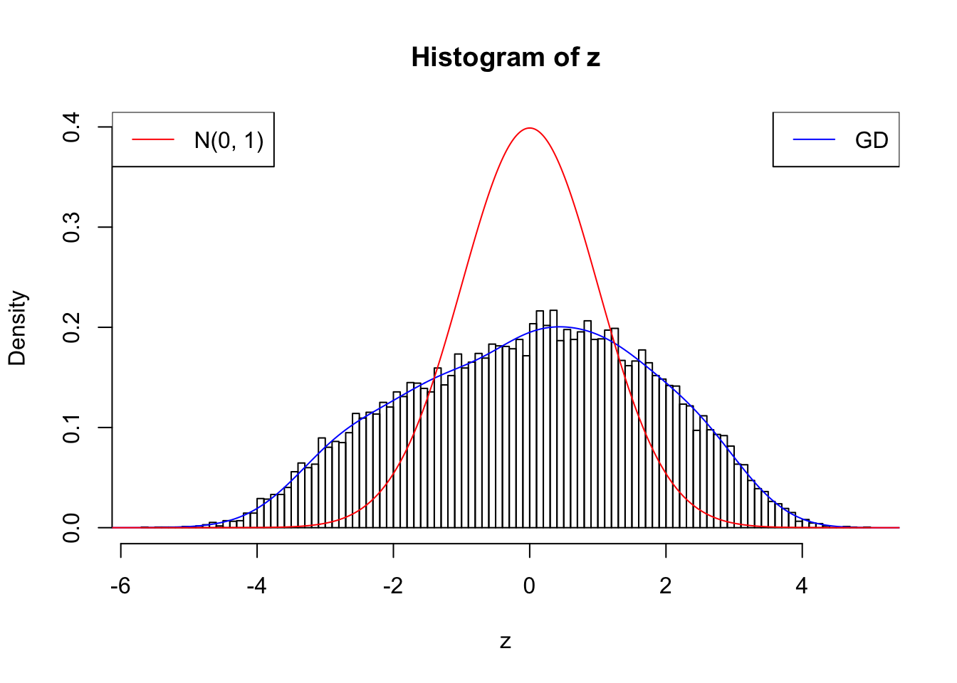
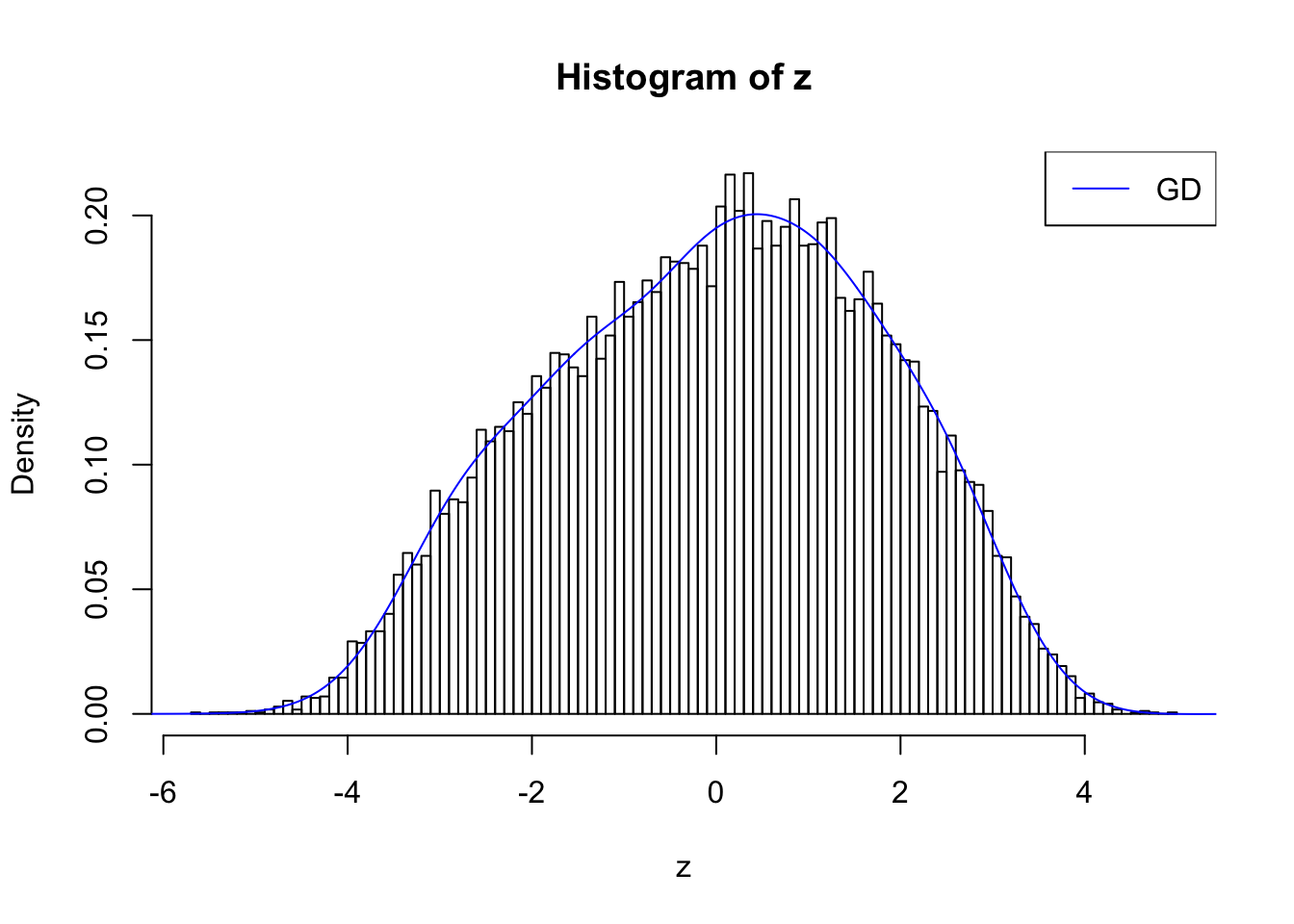
With stretch GD can fit \(z\) scores, but it seems there should be signals.
GD Coefficients:0 : 1 ; 1 : 0.0112765123515512 ; 2 : 1.60751487400088 ; 3 : 0.361378958092869 ; 4 : 1.65789257614746 ; 5 : 0.670189379060472 ; 6 : 0.75997503879673 ; 7 : 0.557659272292024 ; 8 : -0.0586994517219462 ; 9 : 0.175073181131849 ; 10 : -0.132350826272713 ;

Discovered by BH and ASH
Feeding summary statistics to BH and ASH, both give thousands of discoveries.
fit.BH = p.adjust((1 - pnorm(abs(z))) * 2, method = "BH")
## Number of discoveries by BH
sum(fit.BH <= 0.05)
[1] 2541fit.ash = ashr::ash(betahat, sebetahat, method = "fdr")
## Number of discoveries by ASH
sum(get_svalue(fit.ash) <= 0.05)[1] 6440Fitting ASH first or Gaussian derivatives first
Using default setting \(L = 10\), \(\lambda = 10\), \(\rho = 0.5\), compare the GD-ASH results by fitting ASH first vs fitting GD first. They indeed arrive at different local minima.
fit.gdash.ASH <- gdash(betahat, sebetahat,
                       gd.priority = FALSE)
## Regularized log-likelihood by fitting ASH first
fit.gdash.ASH$loglik
[1] -12483.86fit.gdash.GD <- gdash(betahat, sebetahat)
## Regularized log-likelihood by fitting GD first
fit.gdash.GD$loglik[1] -22136.92GD-ASH with larger penalties on \(w\)
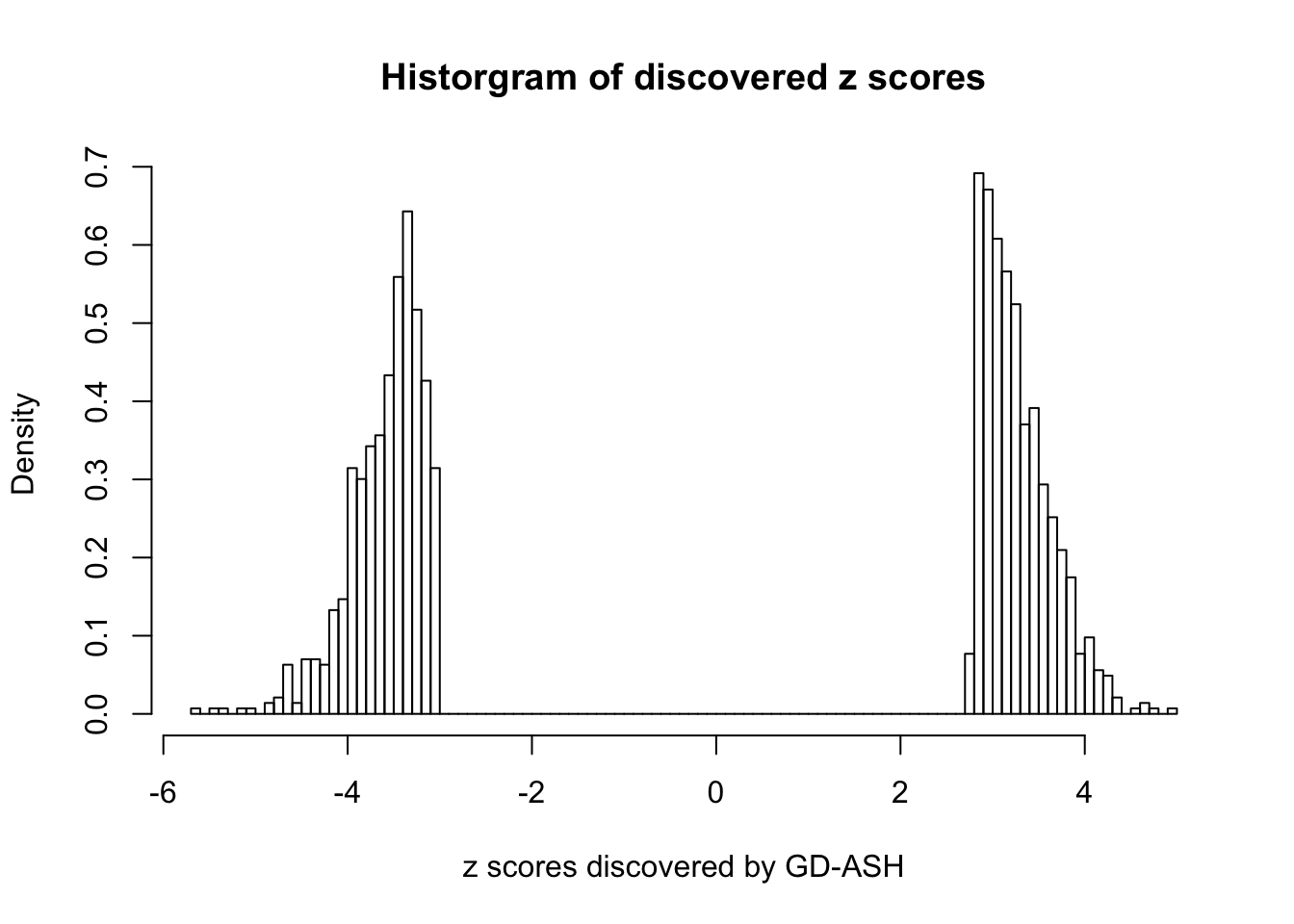
Using \(\lambda = 50\), \(\rho = 0.1\), fitting ASH first and GD first give the same result, and produce 1400+ discoveries with \(q\) values \(\leq 0.05\), all of which are discovered by BH.
L = 10
lambda = 50
rho = 0.1
fit.gdash.ASH <- gdash(betahat, sebetahat,
                       gd.ord = L, w.lambda = lambda, w.rho = rho,
                       gd.priority = FALSE)
## Regularized log-likelihood by fitting ASH first
fit.gdash.ASH$loglik
[1] -13651.59## Number of discoveries
sum(fit.gdash.ASH$qvalue <= 0.05)[1] 1431fit.gdash.GD <- gdash(betahat, sebetahat,
gd.ord = L, w.lambda = lambda, w.rho = rho,
gd.priority = TRUE)
## Regularized log-likelihood by fitting GD first
fit.gdash.GD$loglik[1] -13651.59## Number of discoveries
sum(fit.gdash.GD$qvalue <= 0.05)[1] 1431GD Coefficients:0 : 1 ; 1 : -0.0475544308510135 ; 2 : 0.707888470469342 ; 3 : 0.149489828947119 ; 4 : -8.97499076623316e-14 ; 5 : 0.109281416075664 ; 6 : -3.00530934822662e-13 ; 7 : 0.0783545592042359 ; 8 : -2.99572304462426e-13 ; 9 : 0.0911488252640105 ; 10 : -2.99578347875936e-13 ;
Session information
sessionInfo()R version 3.3.3 (2017-03-06)
Platform: x86_64-apple-darwin13.4.0 (64-bit)
Running under: macOS Sierra 10.12.5
locale:
[1] en_US.UTF-8/en_US.UTF-8/en_US.UTF-8/C/en_US.UTF-8/en_US.UTF-8
attached base packages:
[1] stats graphics grDevices utils datasets methods base
other attached packages:
[1] ashr_2.1-19 Rmosek_7.1.3 PolynomF_0.94 cvxr_0.0.0.9009
[5] REBayes_0.62 Matrix_1.2-8 SQUAREM_2016.10-1 EQL_1.0-0
[9] ttutils_1.0-1
loaded via a namespace (and not attached):
[1] Rcpp_0.12.11 knitr_1.16 magrittr_1.5
[4] edgeR_3.14.0 MASS_7.3-45 pscl_1.4.9
[7] doParallel_1.0.10 lattice_0.20-34 foreach_1.4.3
[10] stringr_1.2.0 tools_3.3.3 parallel_3.3.3
[13] grid_3.3.3 git2r_0.18.0 iterators_1.0.8
[16] htmltools_0.3.6 assertthat_0.2.0 yaml_2.1.14
[19] rprojroot_1.2 digest_0.6.12 codetools_0.2-15
[22] evaluate_0.10 rmarkdown_1.5 limma_3.28.5
[25] stringi_1.1.2 backports_1.0.5 truncnorm_1.0-7 This R Markdown site was created with workflowr