Histograms of correlated \(z\) scores

Introduction

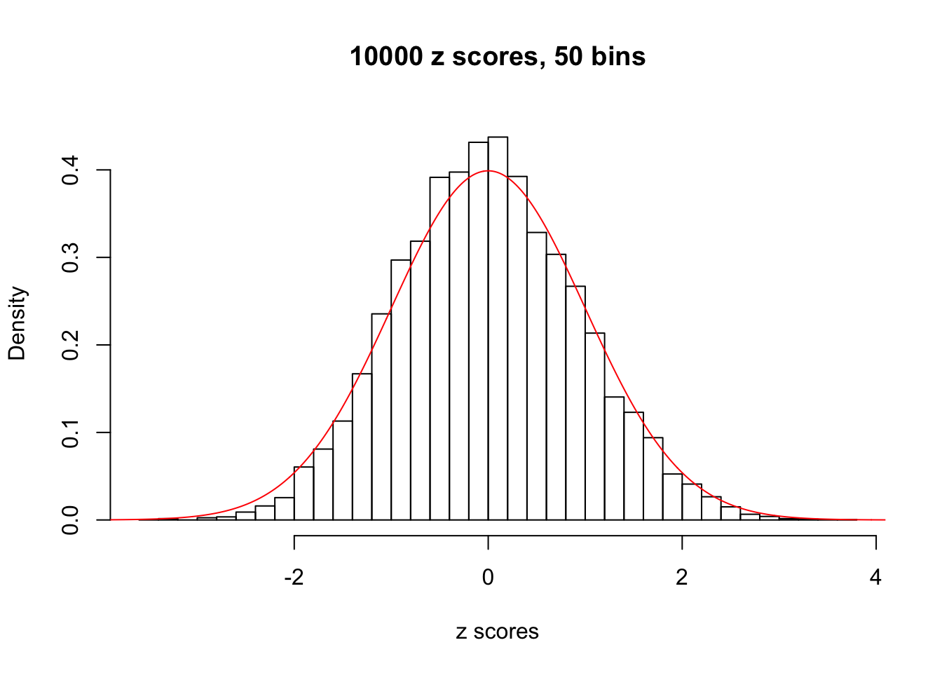
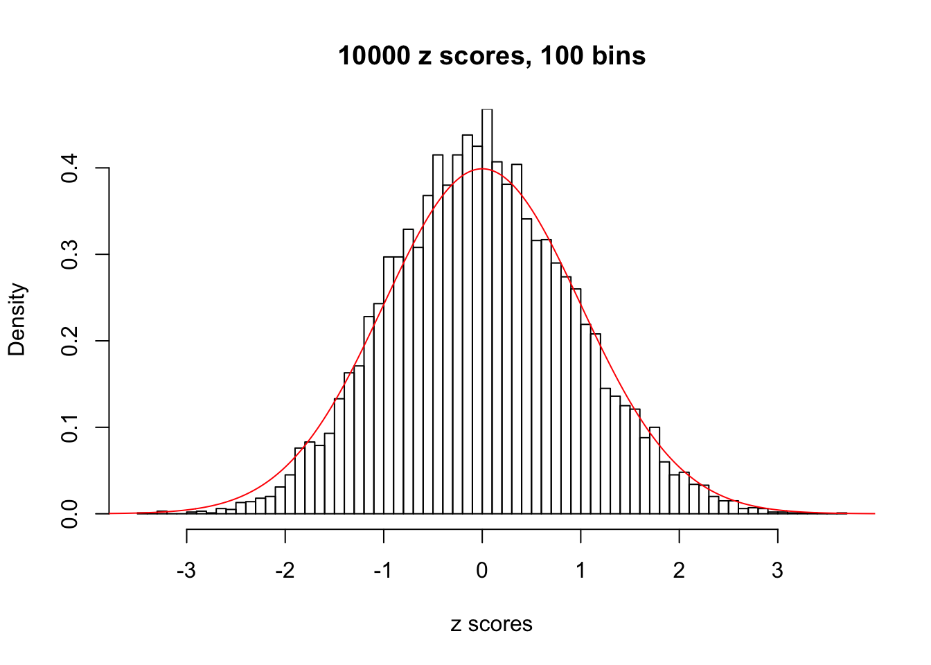
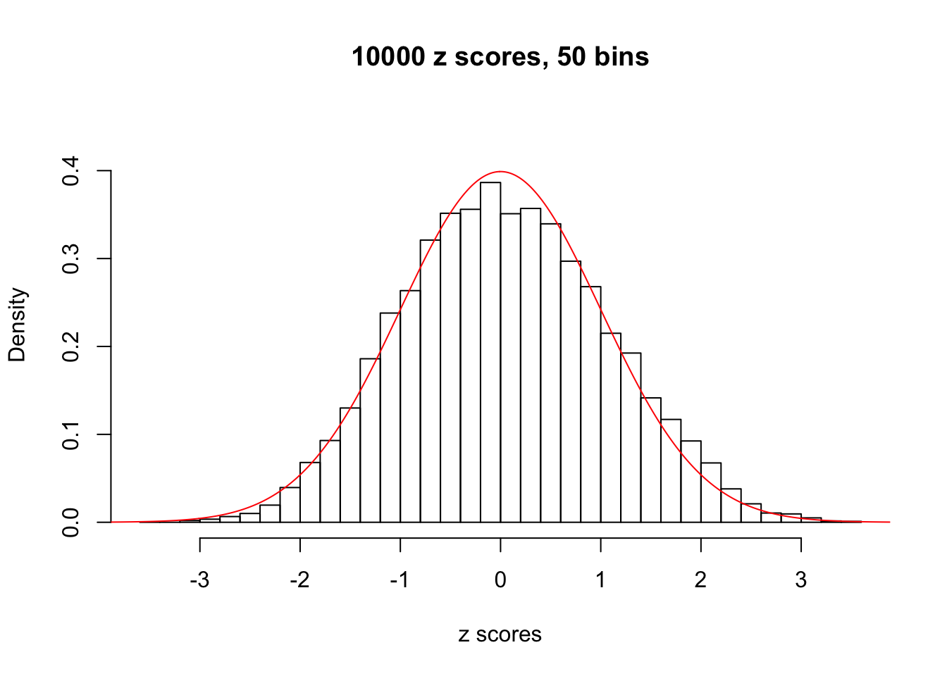
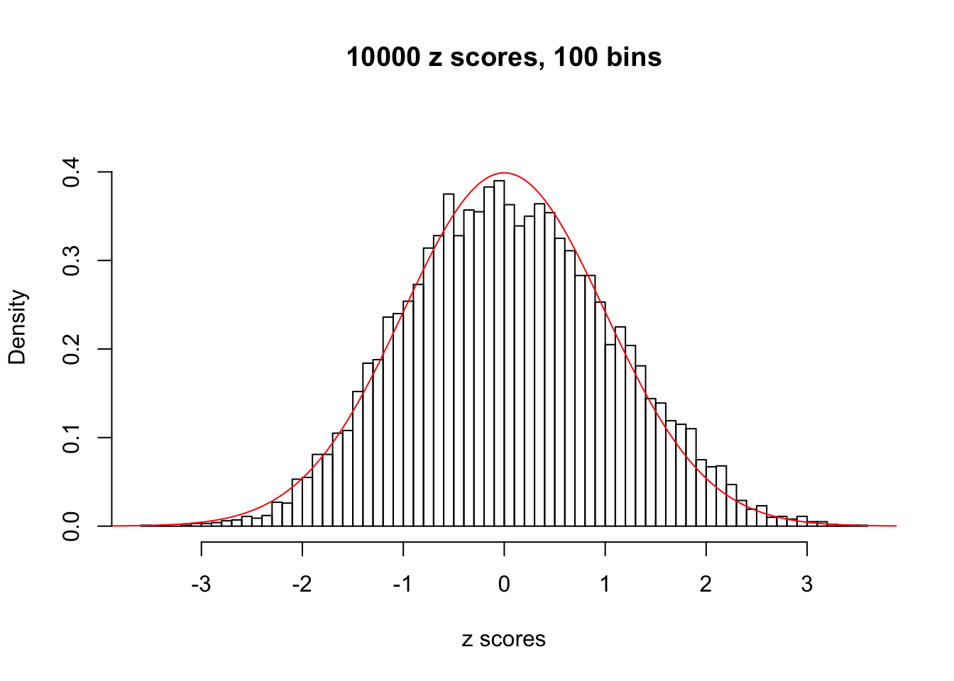
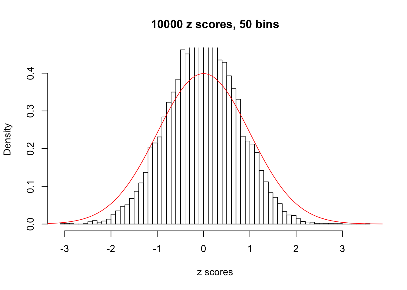
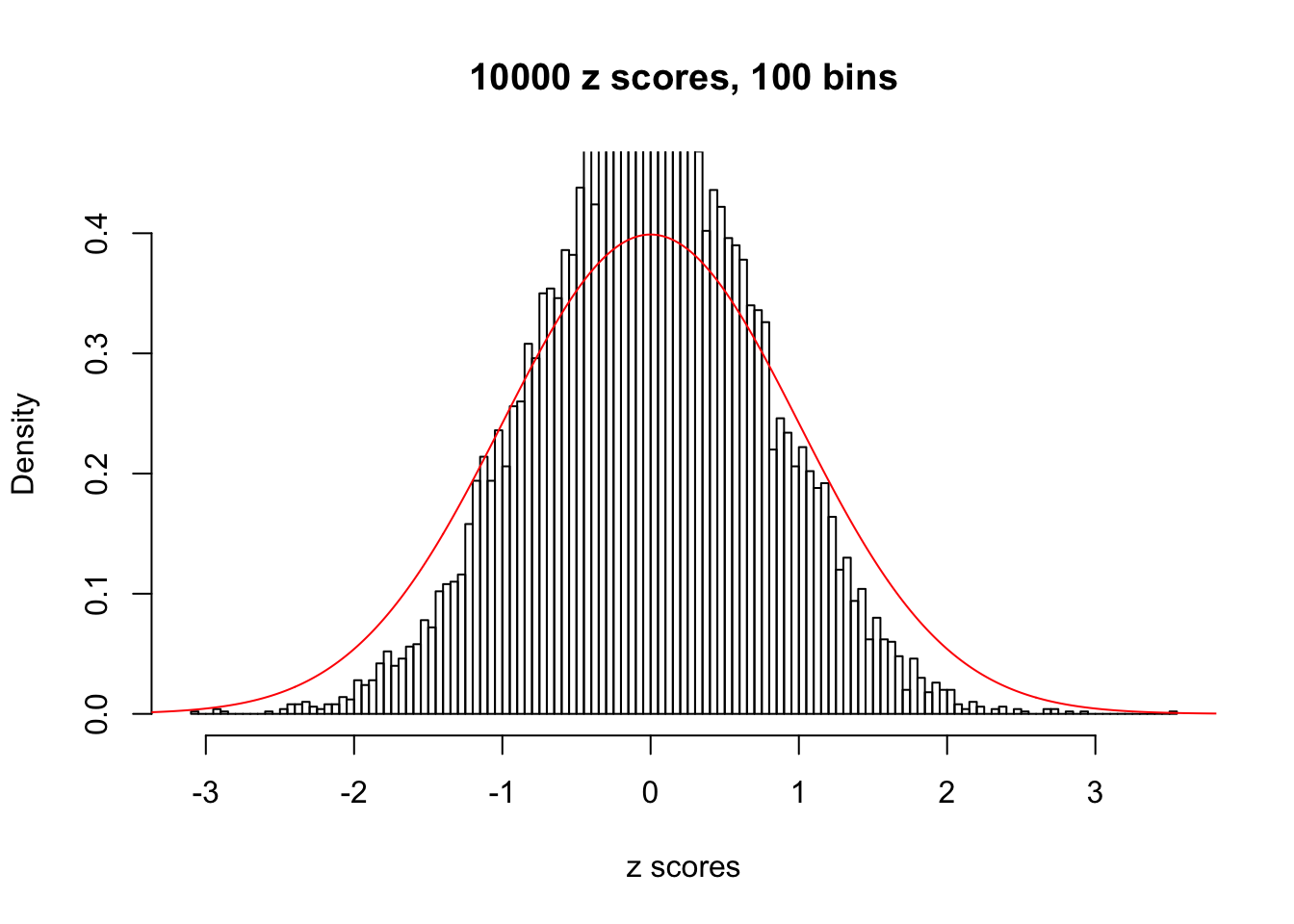
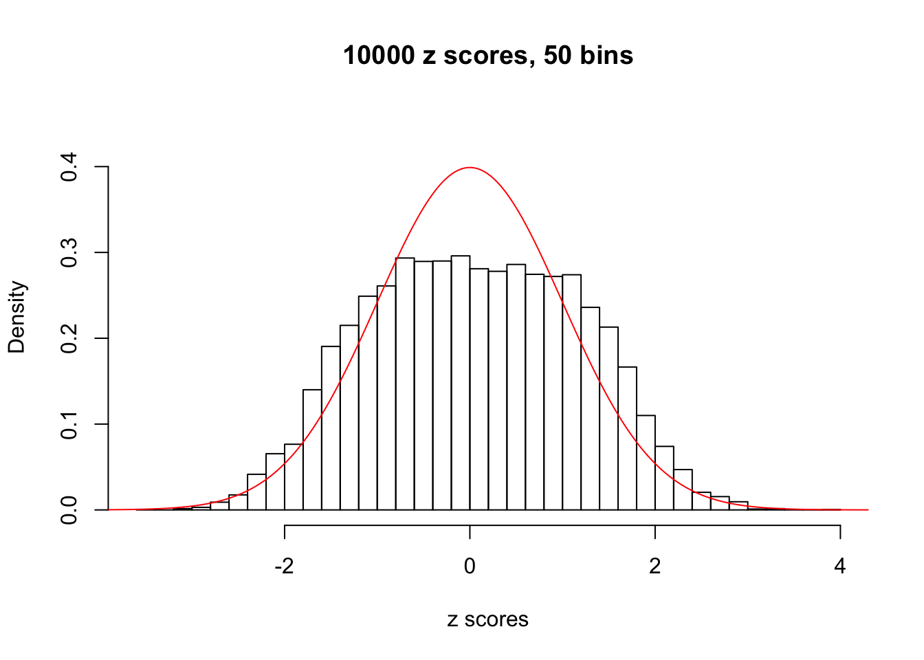
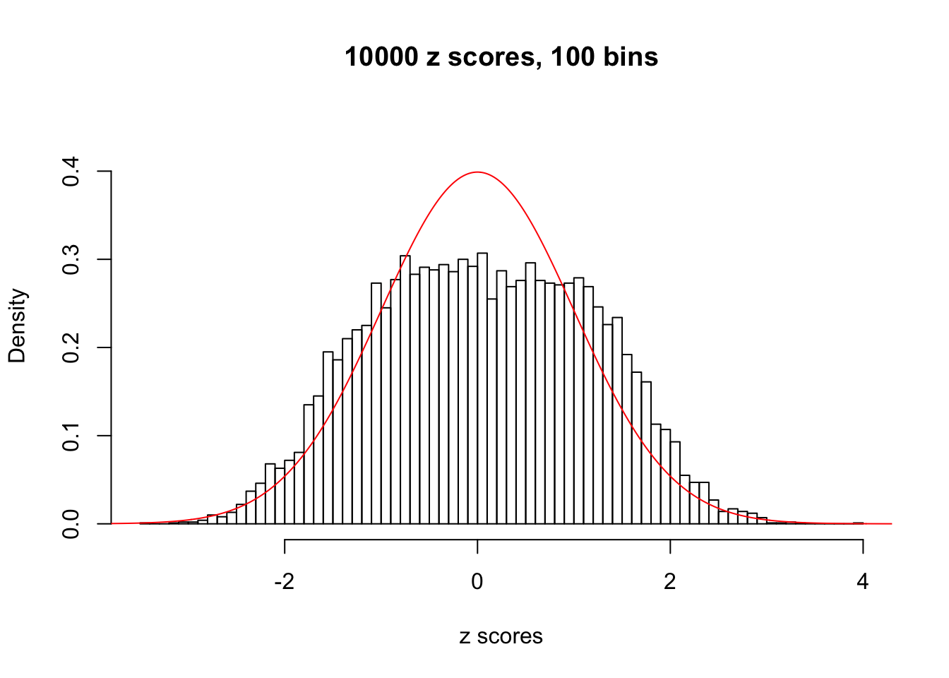
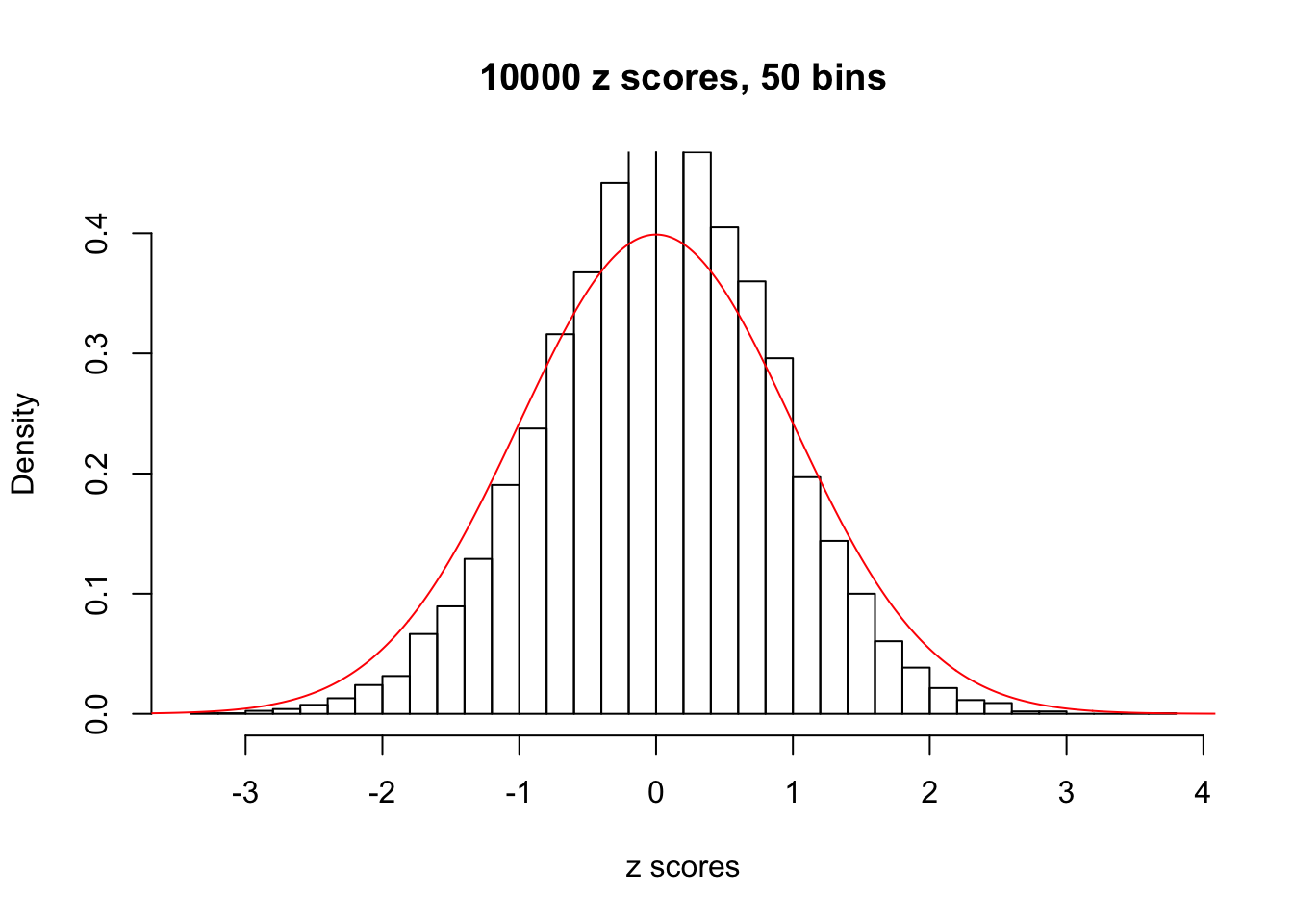
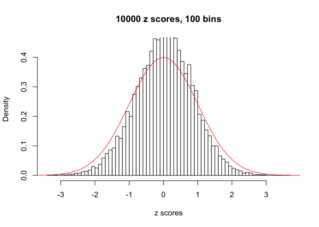
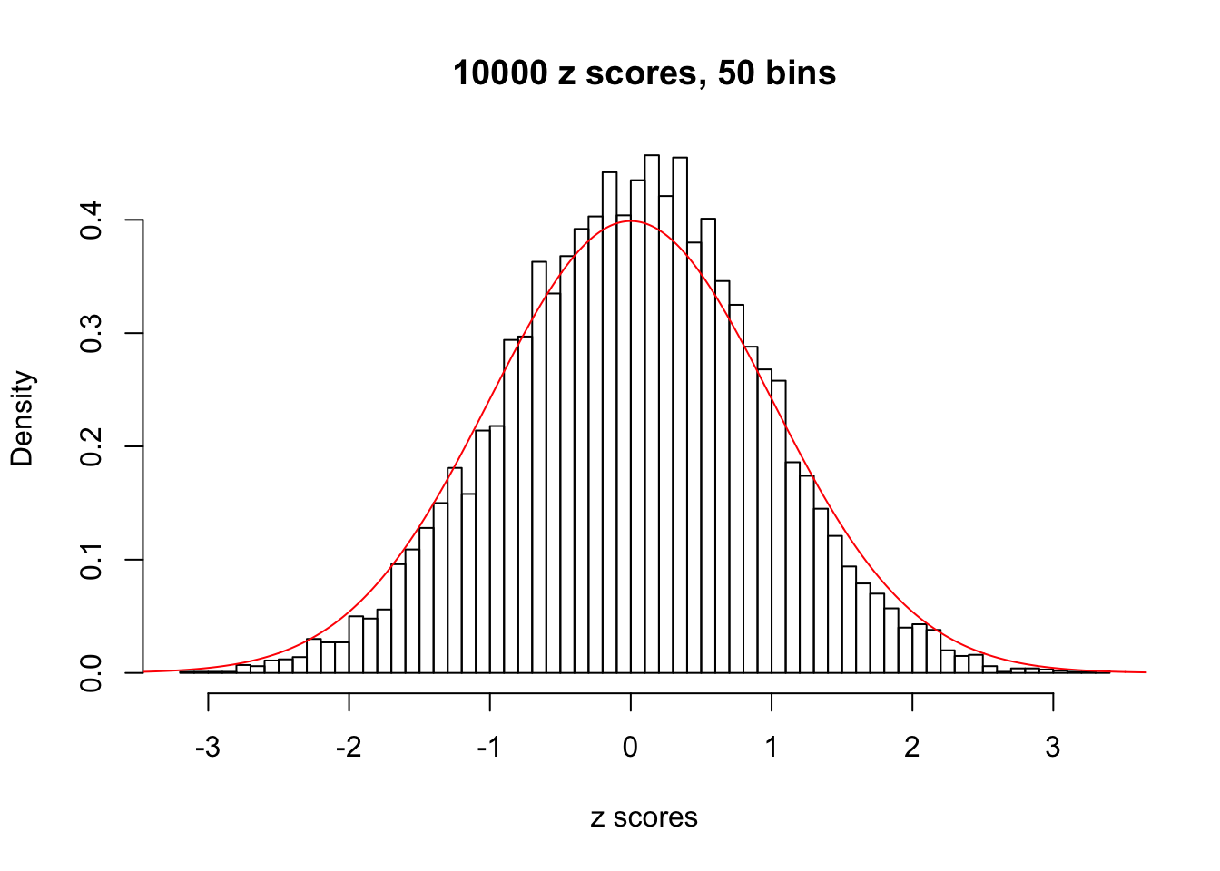
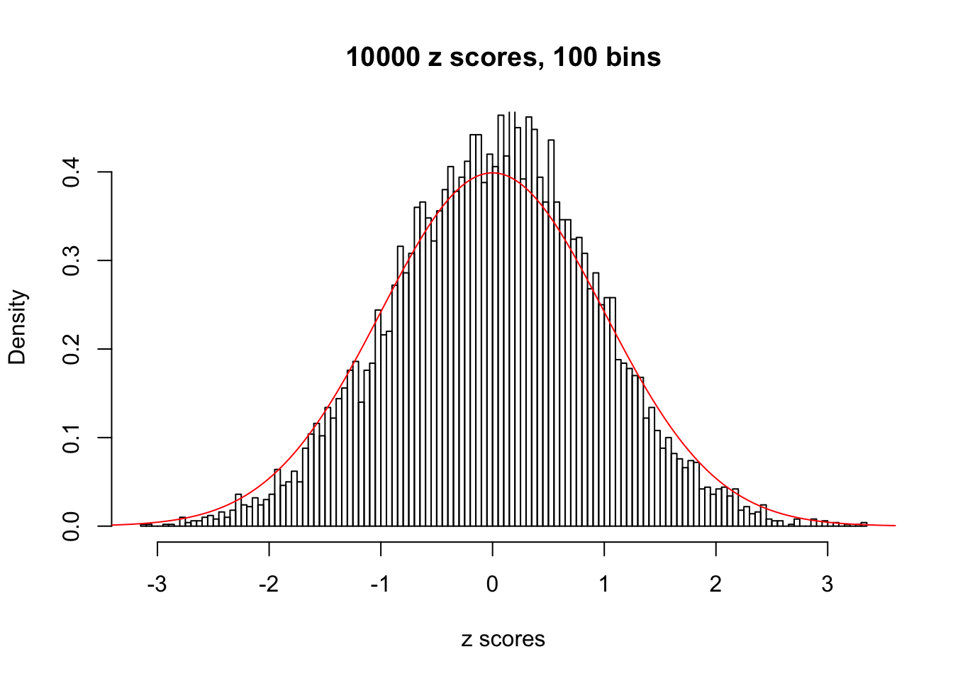
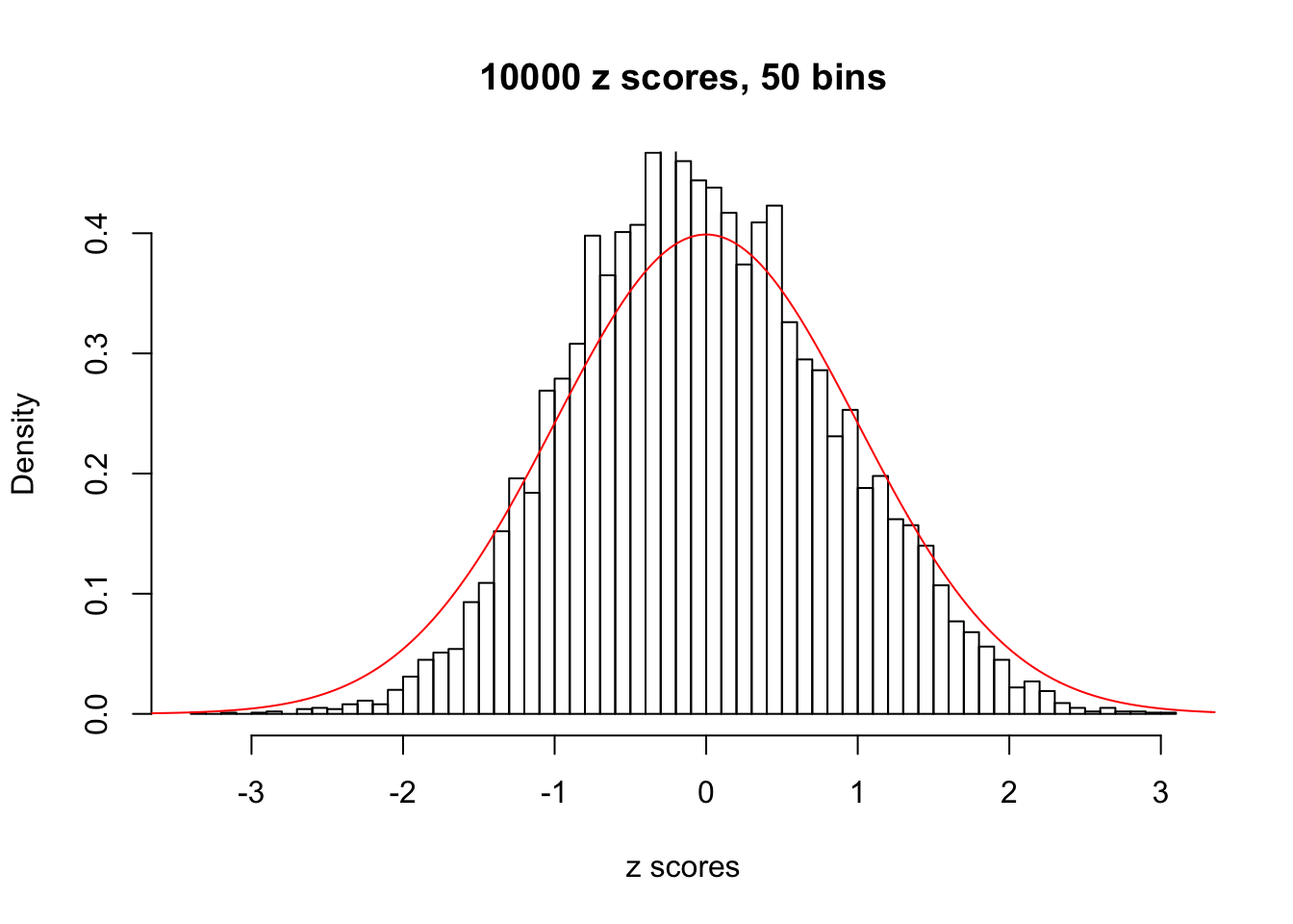
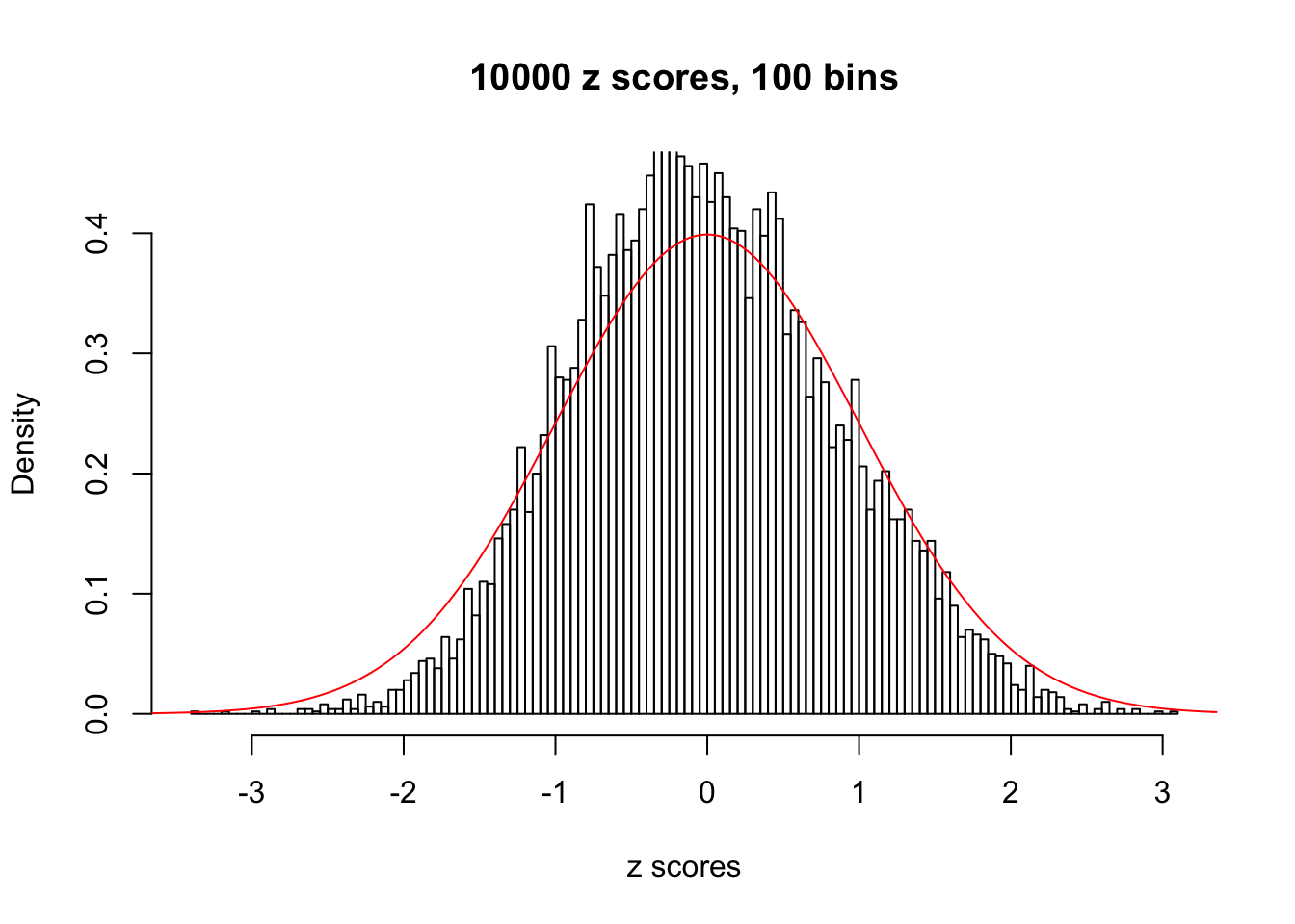
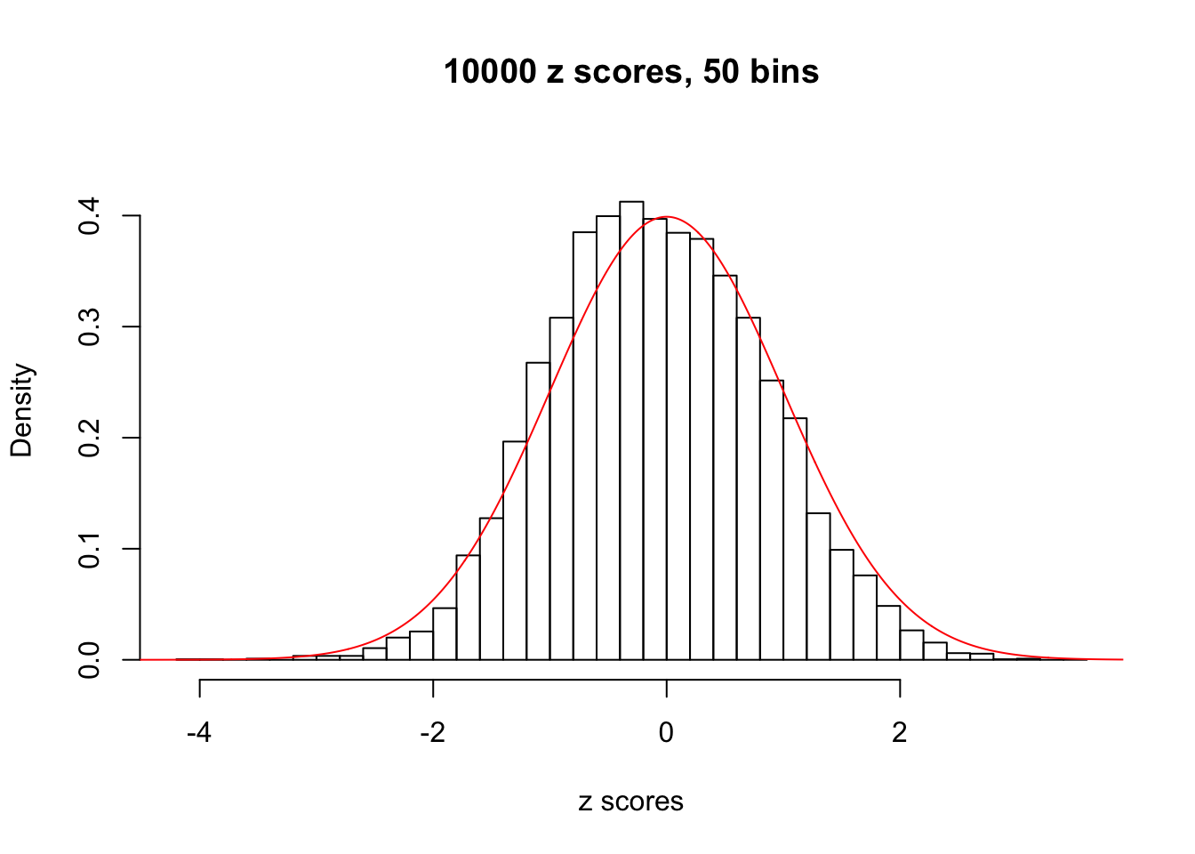
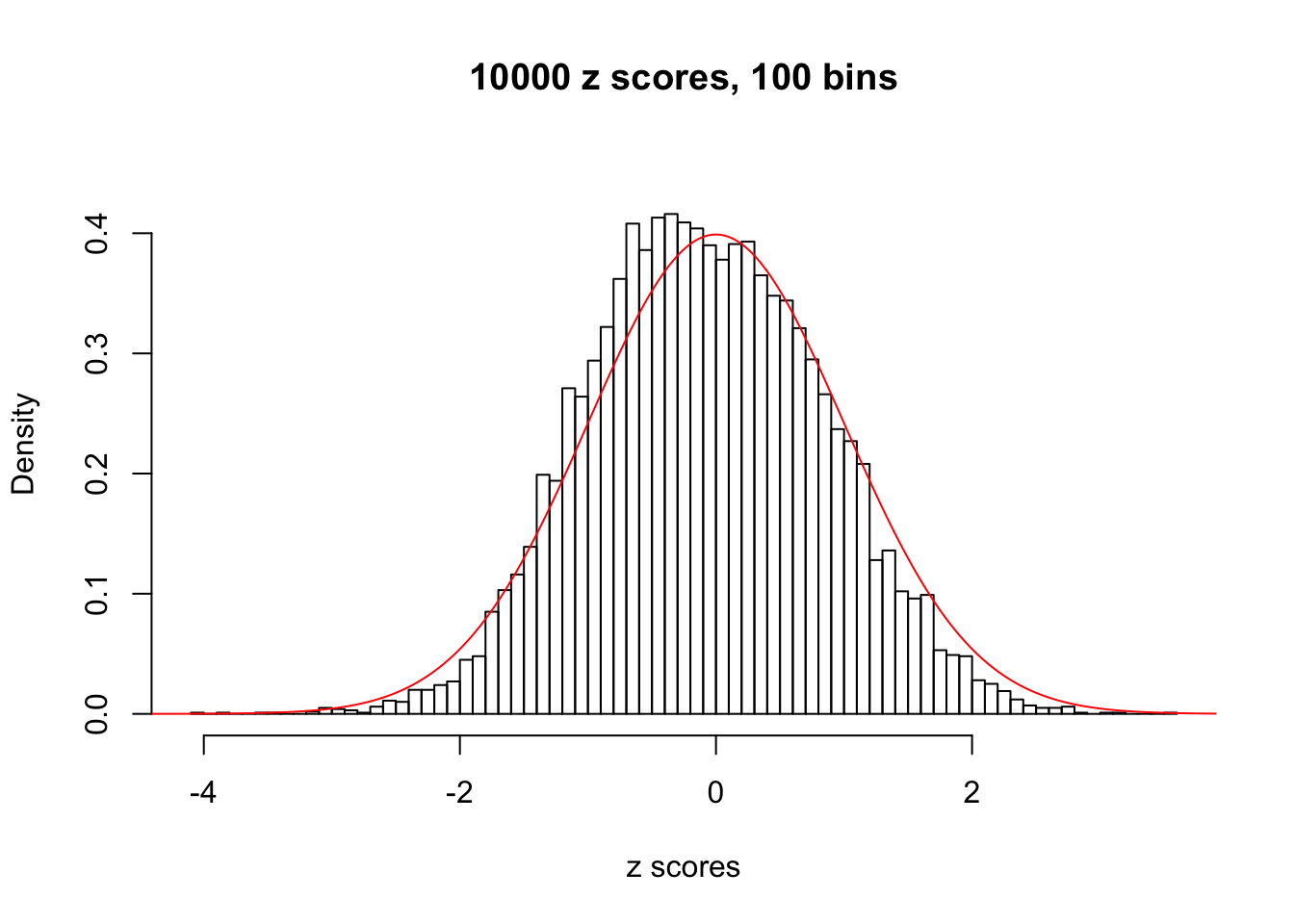
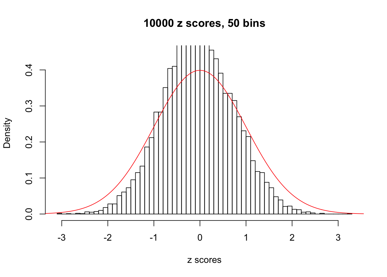
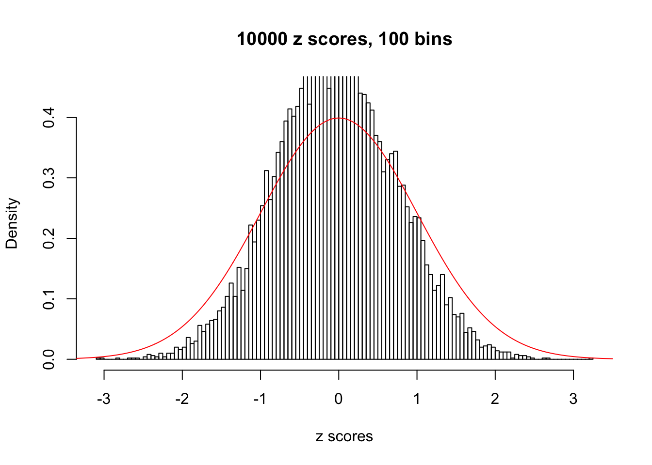
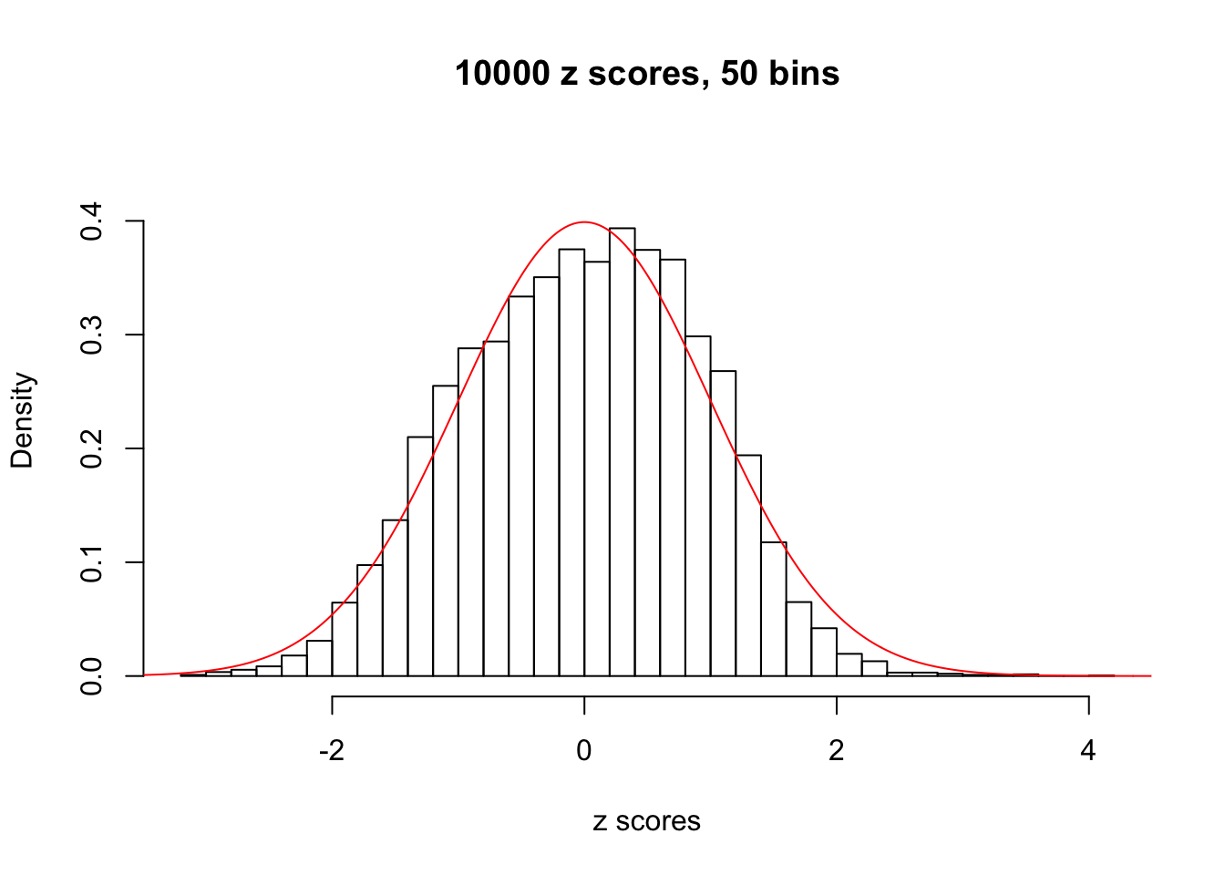
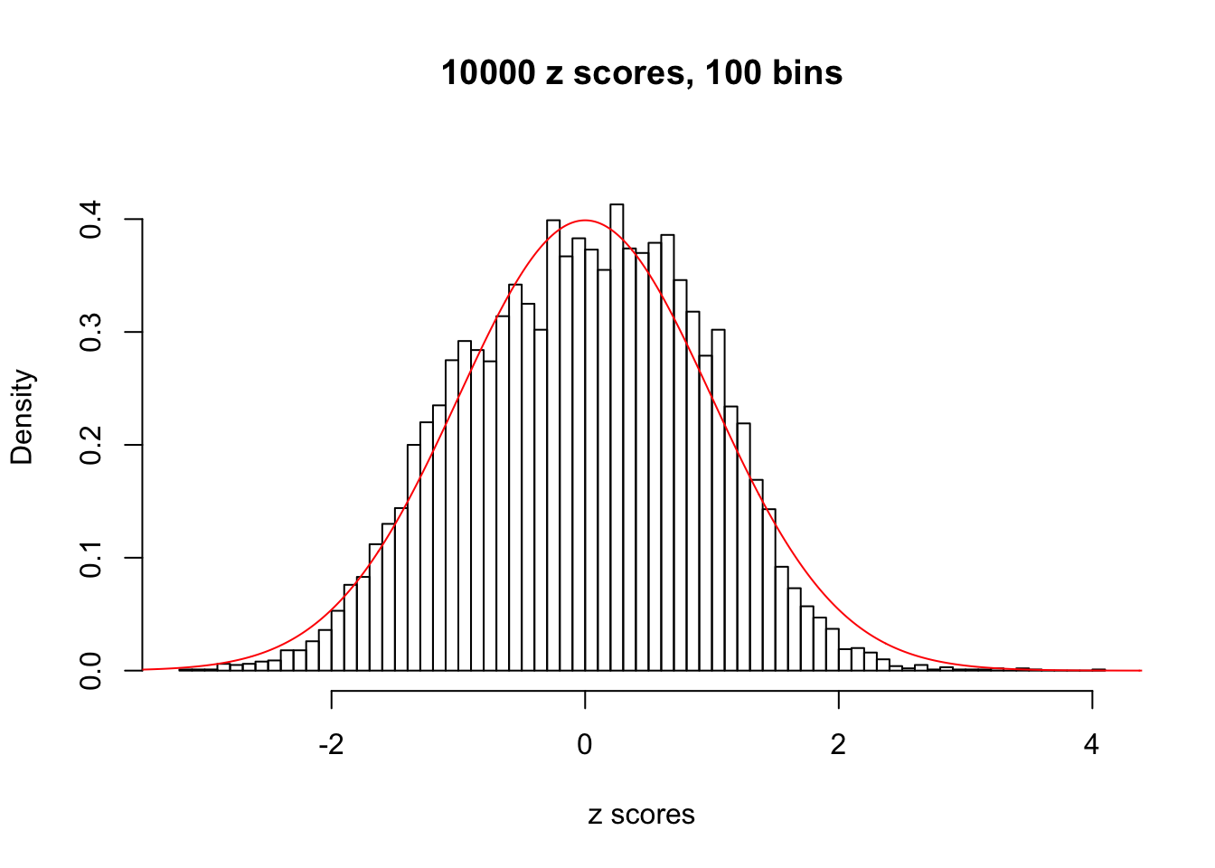
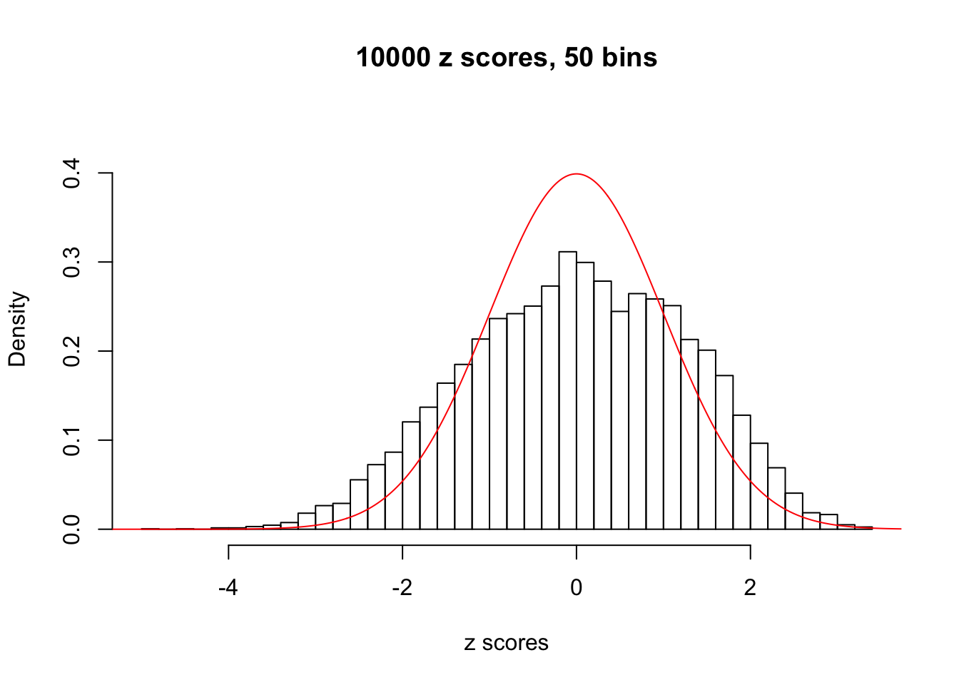
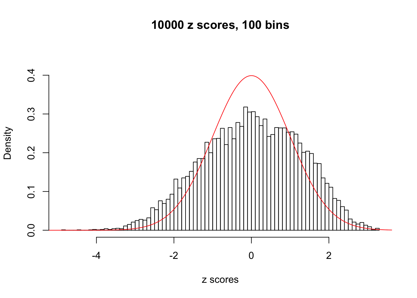
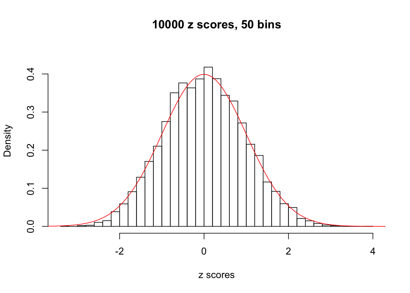
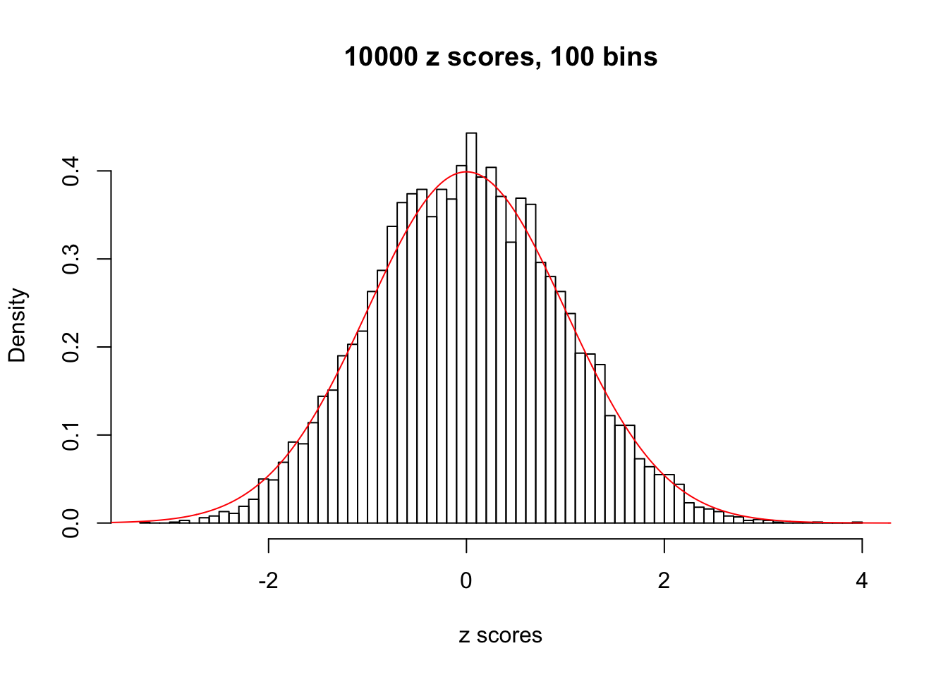
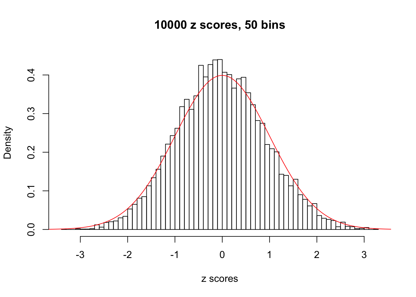
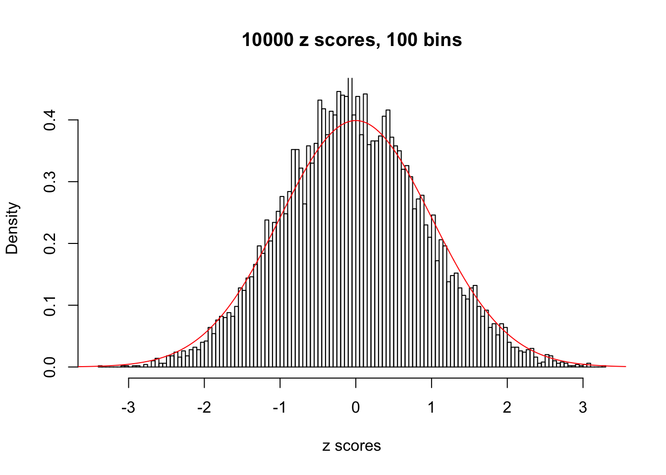
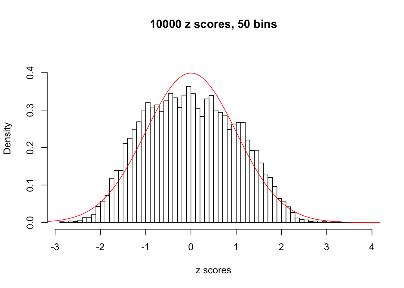
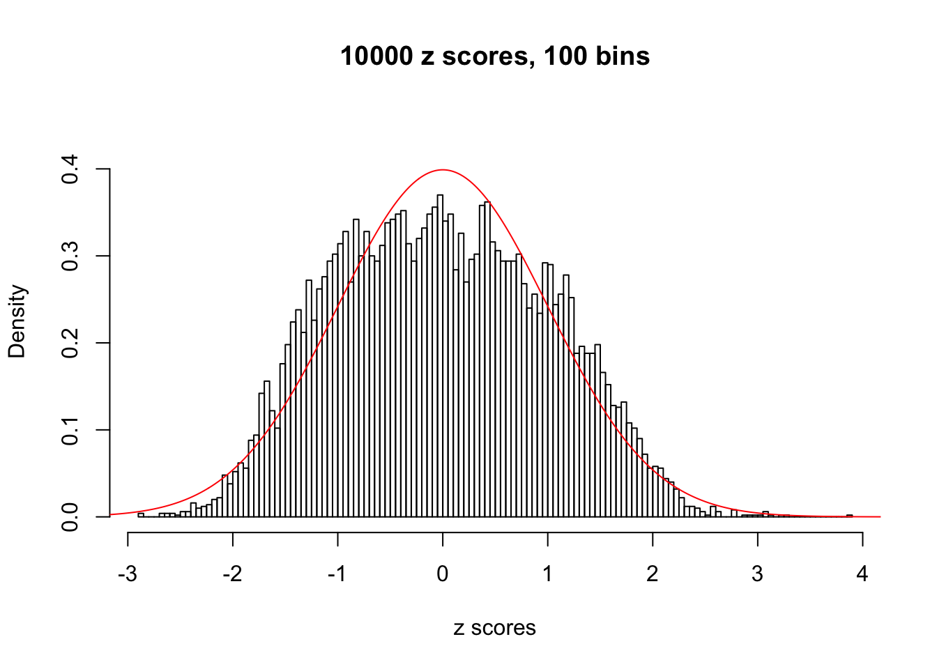
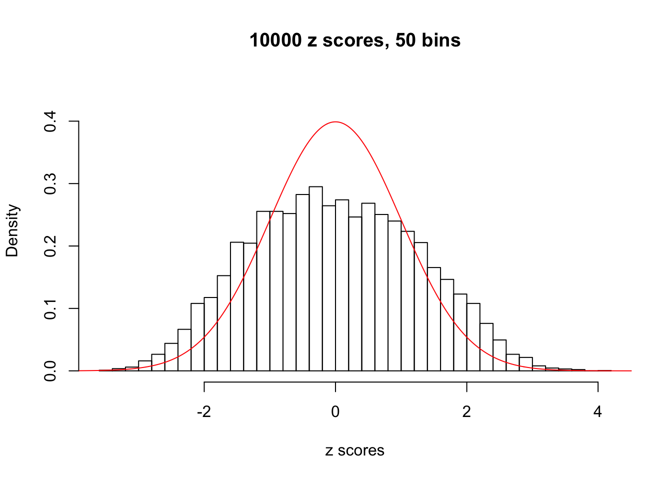
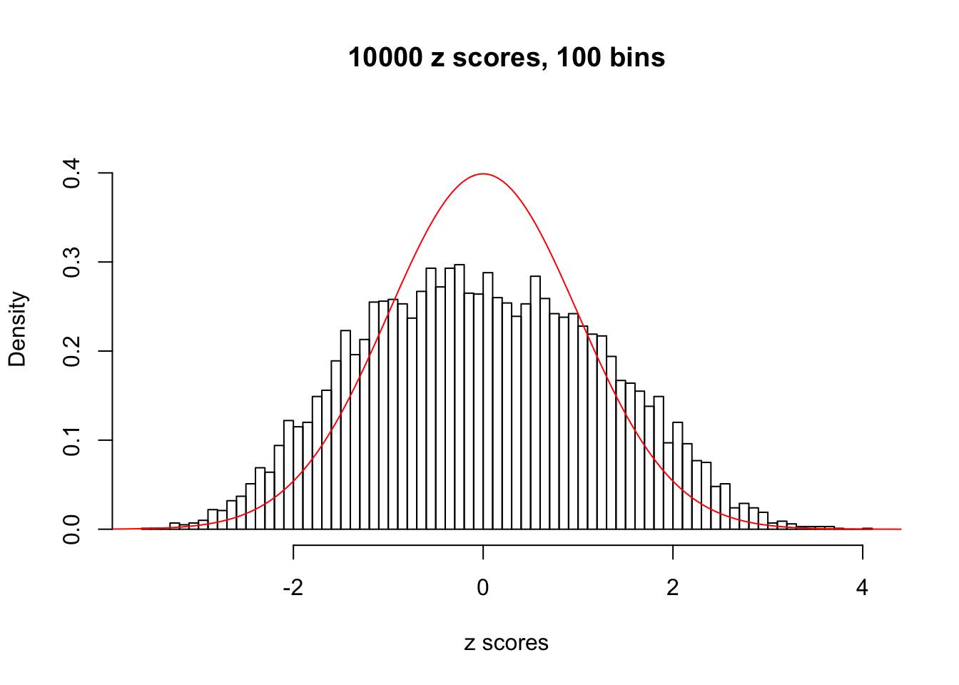
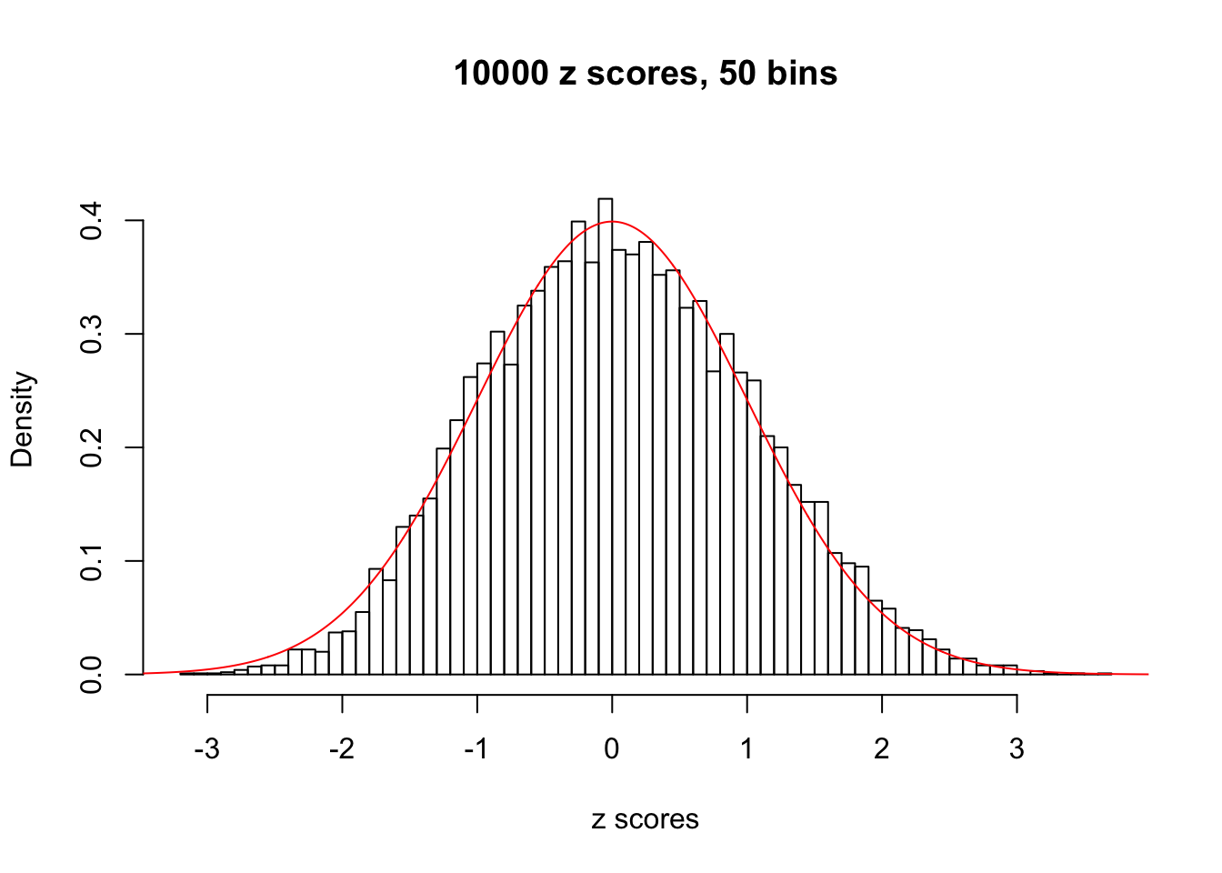
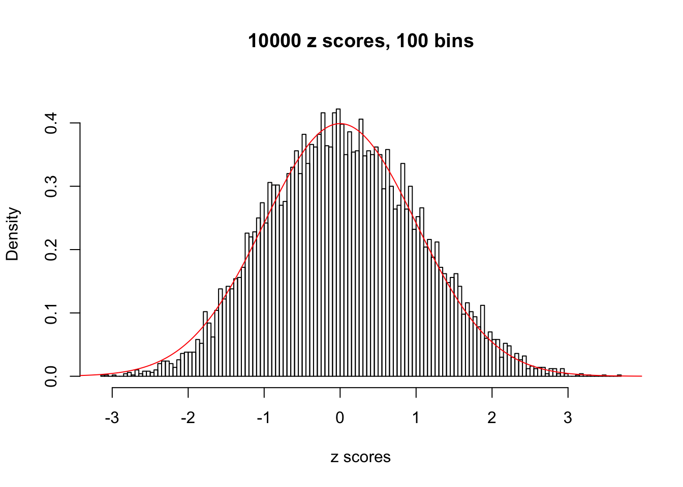
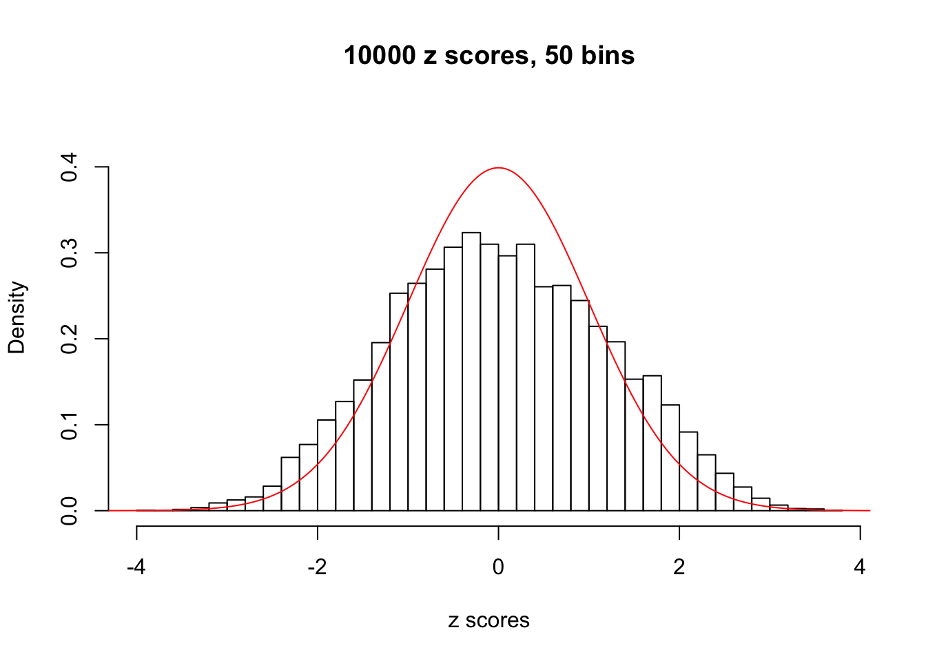
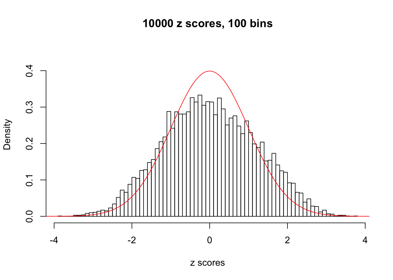
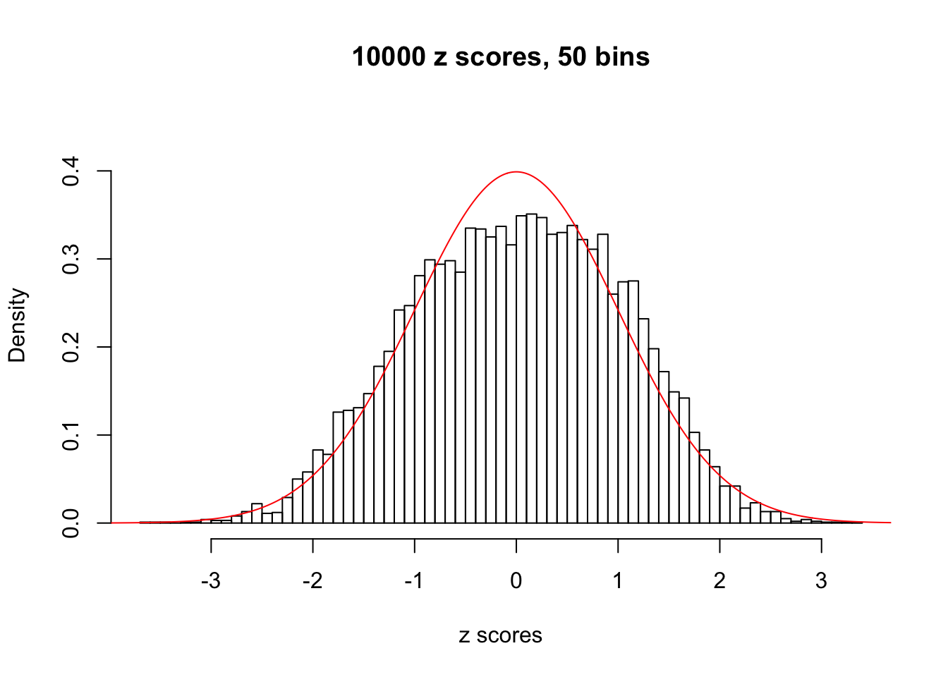
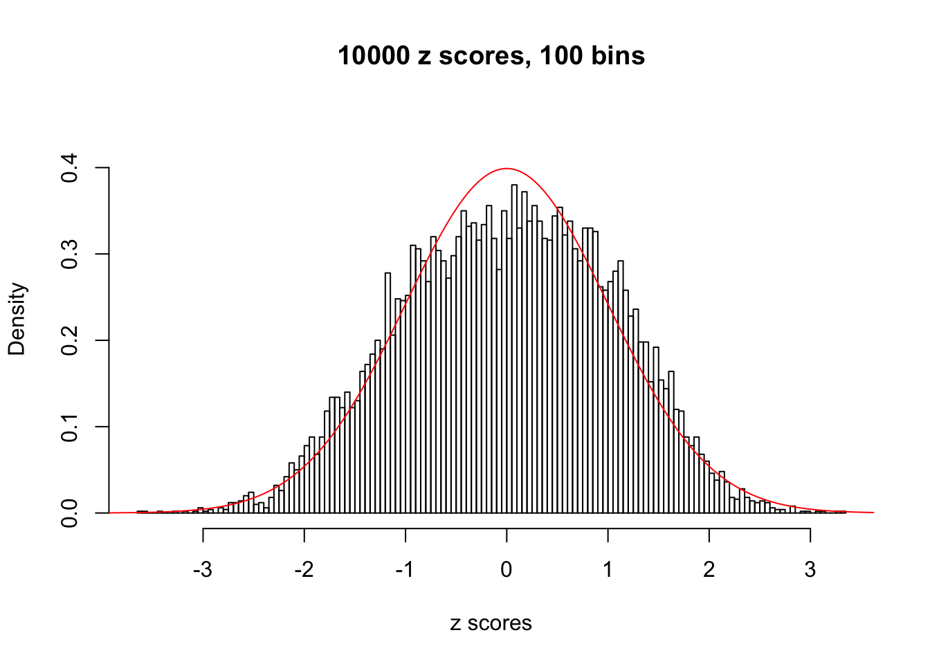
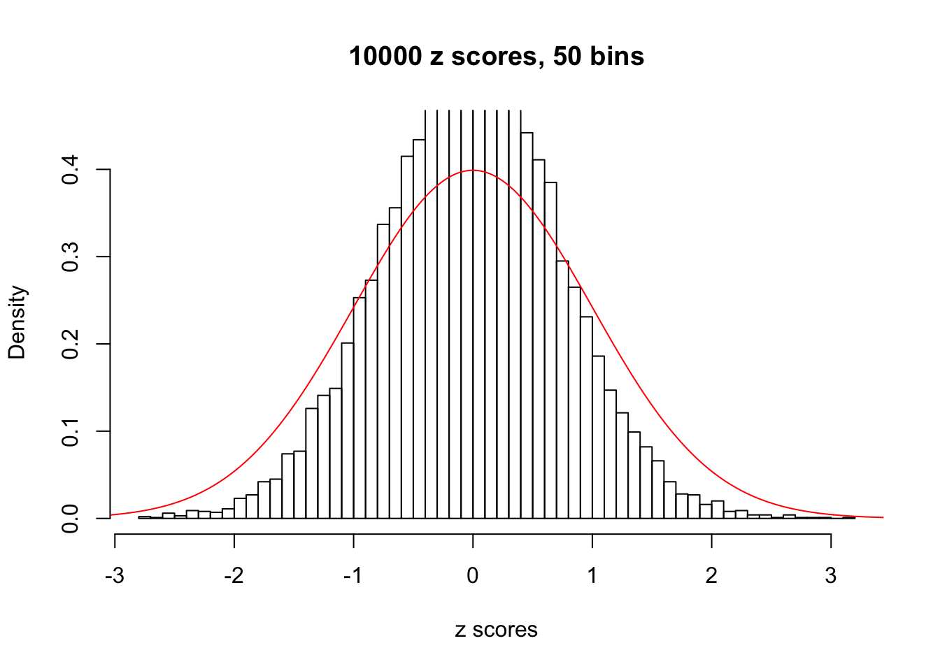
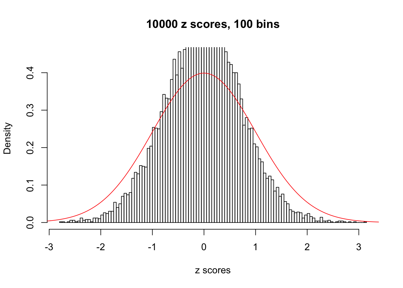
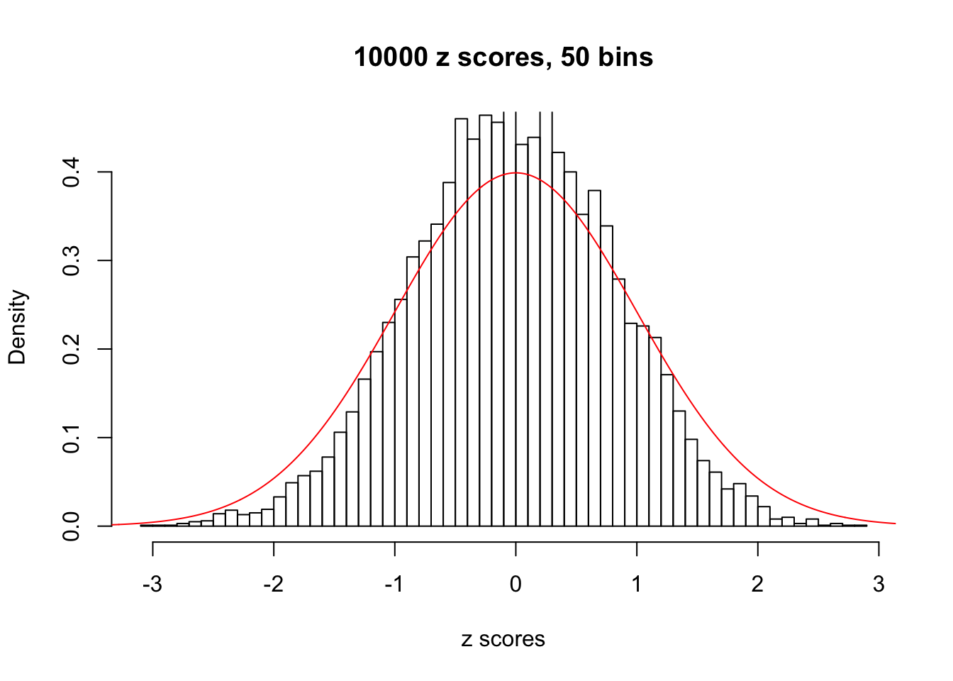
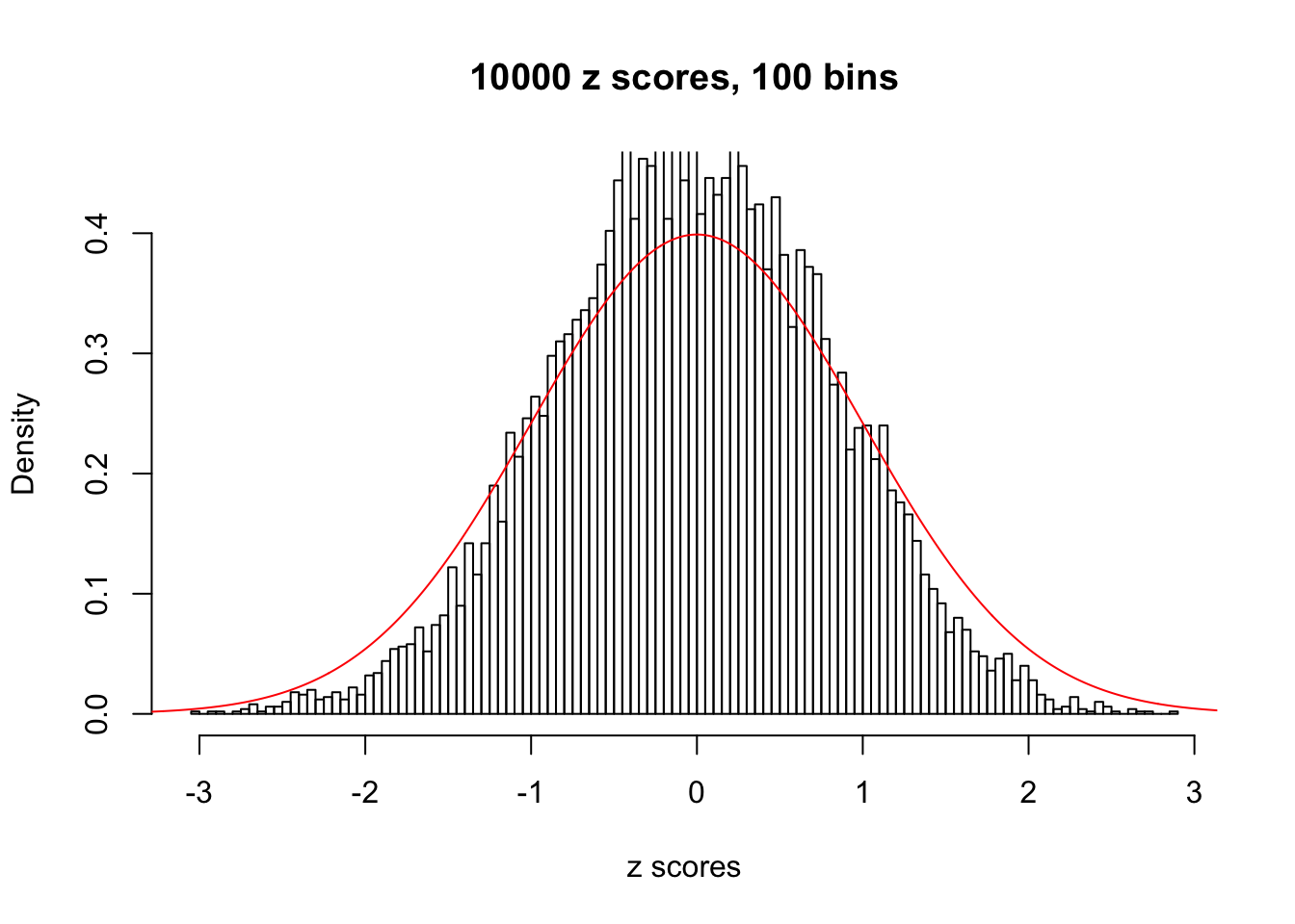
Efron 2010 and Schwartzman’s comment brings to the center the question “what’s the behavior of \(z\) scores under covariance?” Schwartzman pointed out in theory that “the observed histogram is more likely to be narrow than wide, and that it cannot be too wide before it becomes bimodal.” Let’s take a look if this result holds true under our simulation scheme with GTex/Liver data.

Simulation

z = read.table("../output/z_null_liver_777.txt")

sample_z = sample(dim(z)[1], 20)
x = seq(- 10, 10, 0.01)
y = dnorm(x)
for (i in sample_z) {
  hist(as.numeric(z[i, ]), xlab = "z scores", freq = FALSE, ylim = c(0, 0.45), nclass = 50, main = "10000 z scores, 50 bins")
  lines(x, y, col = "red")
  hist(as.numeric(z[i, ]), xlab = "z scores", freq = FALSE, ylim = c(0, 0.45), nclass = 100, main = "10000 z scores, 100 bins")
  lines(x, y, col = "red")
}

Session Information

sessionInfo()

R version 3.3.2 (2016-10-31)
Platform: x86_64-apple-darwin13.4.0 (64-bit)
Running under: macOS Sierra 10.12.3

locale:
[1] en_US.UTF-8/en_US.UTF-8/en_US.UTF-8/C/en_US.UTF-8/en_US.UTF-8

attached base packages:
[1] stats     graphics  grDevices utils     datasets  methods   base     

loaded via a namespace (and not attached):
 [1] backports_1.0.5 magrittr_1.5    rprojroot_1.2   tools_3.3.2    
 [5] htmltools_0.3.5 yaml_2.1.14     Rcpp_0.12.9     stringi_1.1.2  
 [9] rmarkdown_1.3   knitr_1.15.1    git2r_0.18.0    stringr_1.1.0  
[13] digest_0.6.9    workflowr_0.3.0 evaluate_0.10