Empirical Null with Gaussian Derivatives: Perfect Correlation
Lei Sun
2017-03-26
Can \(K\) be too small?
Another assumption to make the problem tractable is that the pairwise correlation \(\rho_{ij}\) is moderate enough so \(W_k\varphi^{(k)}\) vanishes as the order \(k\) increases. With this assumption we can stop at a sufficiently large \(K\) without consideration higher order Gaussian derivatives. But what if \(\rho_{ij}\) is large?
Extreme case: \(\rho_{ij} \equiv 1\)
When we have perfect correlation among all \(z\) scores, the approximate limit observed density \(f_0(x)\to\delta_z(x) = \delta(x-z)\). That is, with probability one, we observe \(z_1 = \cdots = z_n = z\), as \(n\to\infty\), \(f_0(x)\) goes to a Dirac delta function peak at the observed \(z\), and zero elsewhere. Now the question is, can this Dirac delta function be decomposed with the Gaussian \(\varphi\) and its derivatives \(\varphi^{(k)}\), so that we still have
\[ f_0(x) = \delta(x - z) = \varphi(x)\sum\limits_{k = 0}^\infty W_kh_k(x) \] with appropriate \(W_k\)’s?
Using the orthogonality of Hermite functions, we have
\[ W_k = \frac{1}{k!}\int_{-\infty}^{\infty}h_k(x)f_0(x)dx = \frac{1}{k!}\int_{-\infty}^{\infty}h_k(x)\delta(x-z)dx = \frac{1}{k!}h_k(z) \] Now the decomposition \(\varphi(x)\sum\limits_{k = 0}^\infty W_kh_k(x)\) becomes
\[ \varphi(x)\sum\limits_{k = 0}^\infty \frac{1}{k!}h_k(z)h_k(x) \] It turns out this equation is connected to Mehler’s formula which can be shown to give the identity
\[ \sum\limits_{k = 0}^\infty \psi_k(x)\psi_k(z) = \delta(x - z) \] where \(\psi_k\)’s are the Hermite functions defined as
\[ \begin{array}{rrcl} & \psi_k(x) &=& (k!)^{-1/2}(\sqrt{\pi})^{-1/2}e^{-x^2/2}h_k(\sqrt{2}x)\\ \Rightarrow & h_k(x) &=& (k!)^{1/2}(\sqrt{\pi})^{1/2}e^{x^2/4}\psi_k\left(\frac x{\sqrt{2}}\right)\\ \Rightarrow & \varphi(x)\sum\limits_{k = 0}^\infty \frac{1}{k!}h_k(z)h_k(x) & =& \frac1{\sqrt{2}}e^{-\frac{x^2}4+\frac{z^2}4}\sum\limits_{k = 0}^\infty \psi_k\left(\frac x{\sqrt{2}}\right)\psi_k\left(\frac z{\sqrt{2}}\right)\\ & &=& \frac1{\sqrt{2}}e^{-\frac{x^2}4+\frac{z^2}4} \delta\left(\frac{x - z}{\sqrt{2}}\right) \end{array} \] Note that the Dirac delta function has a property that \(\delta(\alpha x) = \delta(x) / |\alpha| \Rightarrow \frac1{\sqrt{2}}\delta\left(\frac{x - z}{\sqrt{2}}\right) = \delta(x - z)\). Therefore,
\[ \varphi(x)\sum\limits_{k = 0}^\infty \frac{1}{k!}h_k(z)h_k(x) = \delta(x-z)\exp\left(-\frac{x^2}4+\frac{z^2}4\right) \] Note that \(\exp\left(-\frac{x^2}4+\frac{z^2}4\right)\) is bounded for any \(z\in\mathbb{R}\), so \(\delta(x-z)\exp\left(-\frac{x^2}4+\frac{z^2}4\right)\) vanishes to \(0\) for any \(x\neq z\), and
\[ \int_{-\infty}^\infty \delta(x-z)\exp\left(-\frac{x^2}4+\frac{z^2}4\right)dx = \exp\left(-\frac{z^2}4+\frac{z^2}4\right) = 1 \] Hence, in essence, \(\delta(x-z)\exp\left(-\frac{x^2}4+\frac{z^2}4\right) = \delta(x-z)\). Therefore we have \[ f_0(x) = \varphi(x)\sum\limits_{k = 0}^\infty W_kh_k(x) = \varphi(x)\sum\limits_{k = 0}^\infty \frac{1}{k!}h_k(z)h_k(x) =\delta(x -z) \] when \[ W_k = \frac{1}{k!}h_k(z) \] Thus we show that the Dirac delta function can be decomposed by Gaussian density and its derivatives.
Visualization with finite \(K\)
With Gaussian and its infinite orders of derivatives, we can compose a Dirac delta function at any position, yet what happens if we stop at a finite \(K\)? Let \(f_0^K\) be the approximation of \(f_0 = \delta_z\) with first \(K\) Gaussian derivatives. That is,
\[ f_0^K(x) = \varphi(x)\sum\limits_{k = 0}^K \frac{1}{k!}h_k(z)h_k(x) \ . \] Meanwhile, let \(F_0^K(x) = \int_{-\infty}^x f_0^K(u)du\). It’s easy to shown that
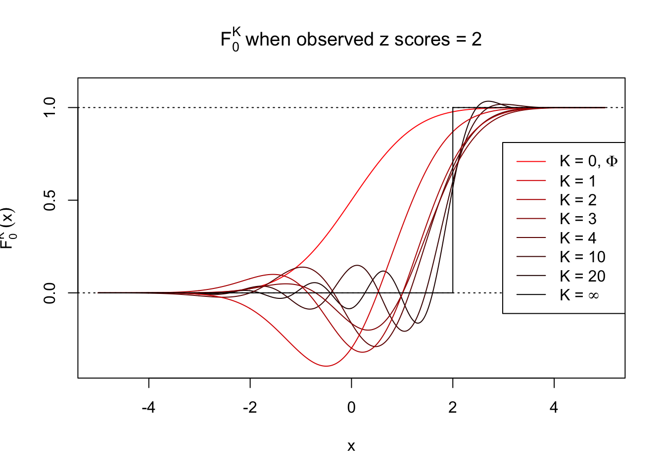
\[ F_0^K(x) = \Phi(x) - \varphi(x)\sum\limits_{k = 1}^K W_k h_{k - 1}(x) = \Phi(x) - \varphi(x) \sum\limits_{k = 1}^K \frac{1}{k!}h_k(z) h_{k - 1}(x) \ . \]
Theoretically, \(f_0^K\) is an approximation to empirical density of perfectly correlated \(z\) scores; hence, as \(K\to\infty\), \(f_0^K\to\delta_z\). Similarly, \(F_0^K\) is an approximation to empirical cdf of perfectly correlated \(z\) scores; hence, as \(K\to\infty\), \(f_0^K\) should converge to the \(0\)-\(1\) step function, and the location of the step is the observed \(z\).
In practice, the convergence is not fast. As we can see from the following visualization, the difference between \(f_0^K\) and \(\delta_z\), as well as that between \(F_0^K\) and the step function, is still conspicuous even if \(K = 20\), which is about the highest order R can reasonbly handle in the current implementation. Therefore, at least in theory it’s possible that \(K\) can be too small.
Note that the oscillation near the presumptive step may be connected with Gibbs phenomenon.
Under perfect correlation, observed z scores = -1 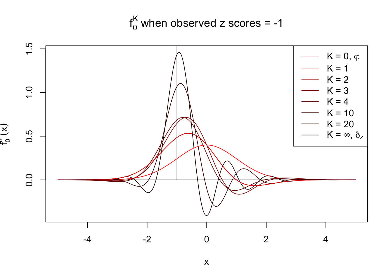
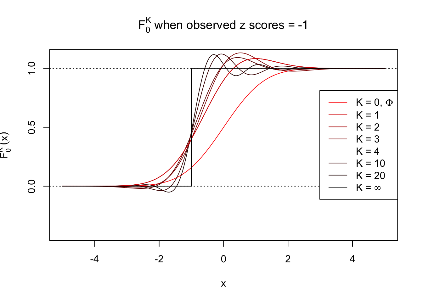
Under perfect correlation, observed z scores = 0 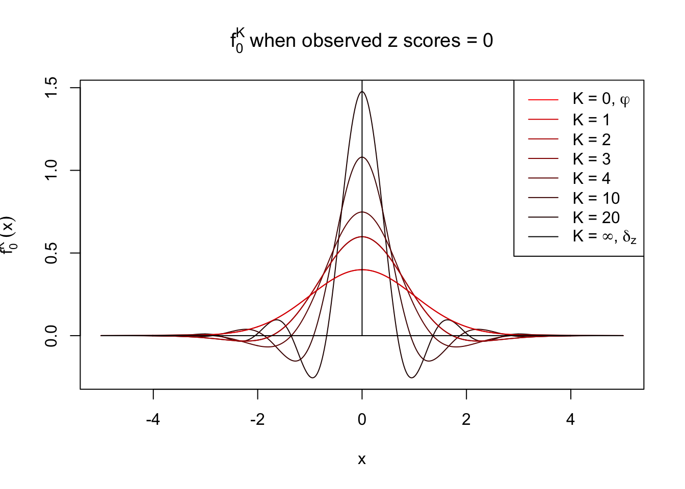
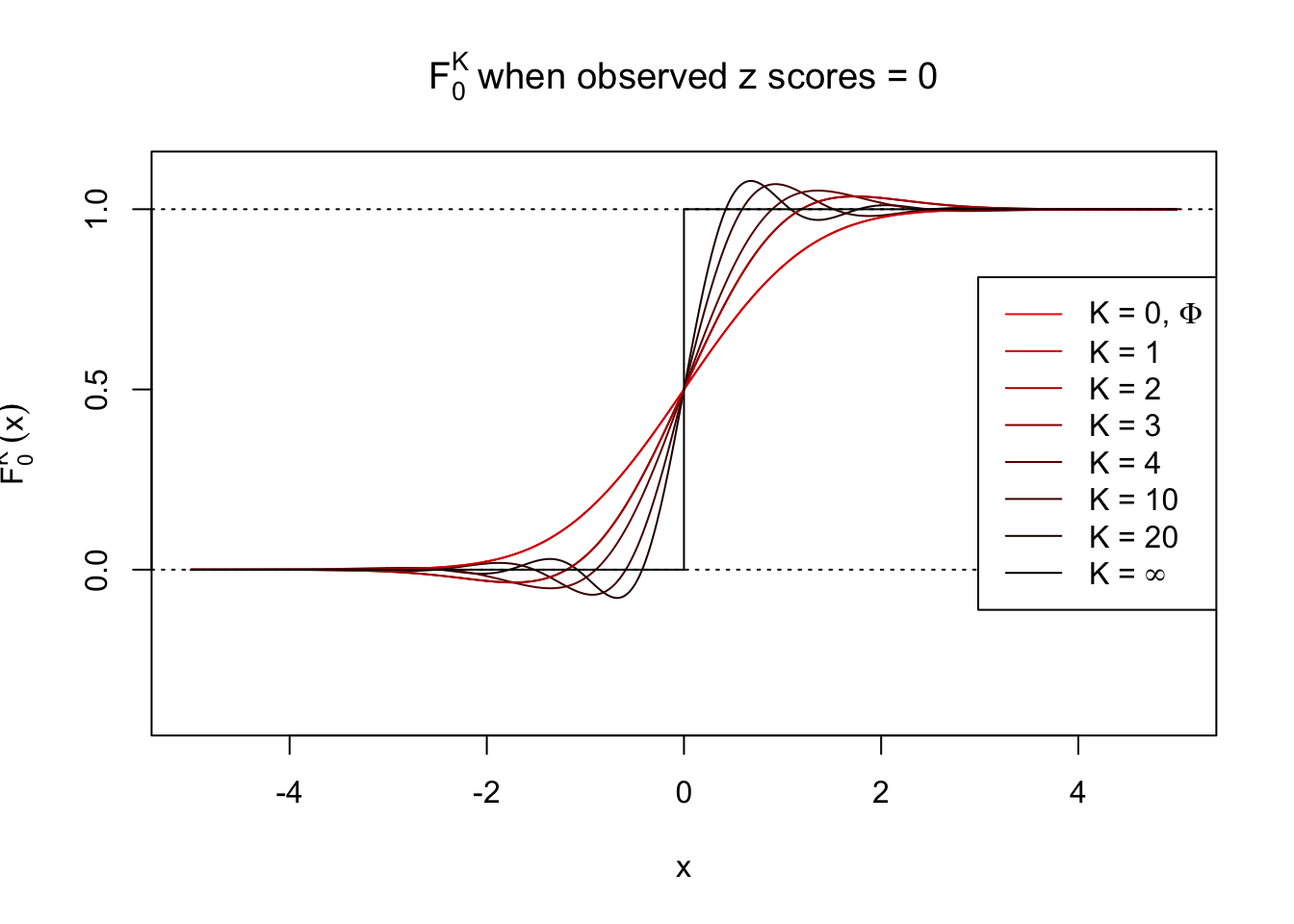
Under perfect correlation, observed z scores = 2 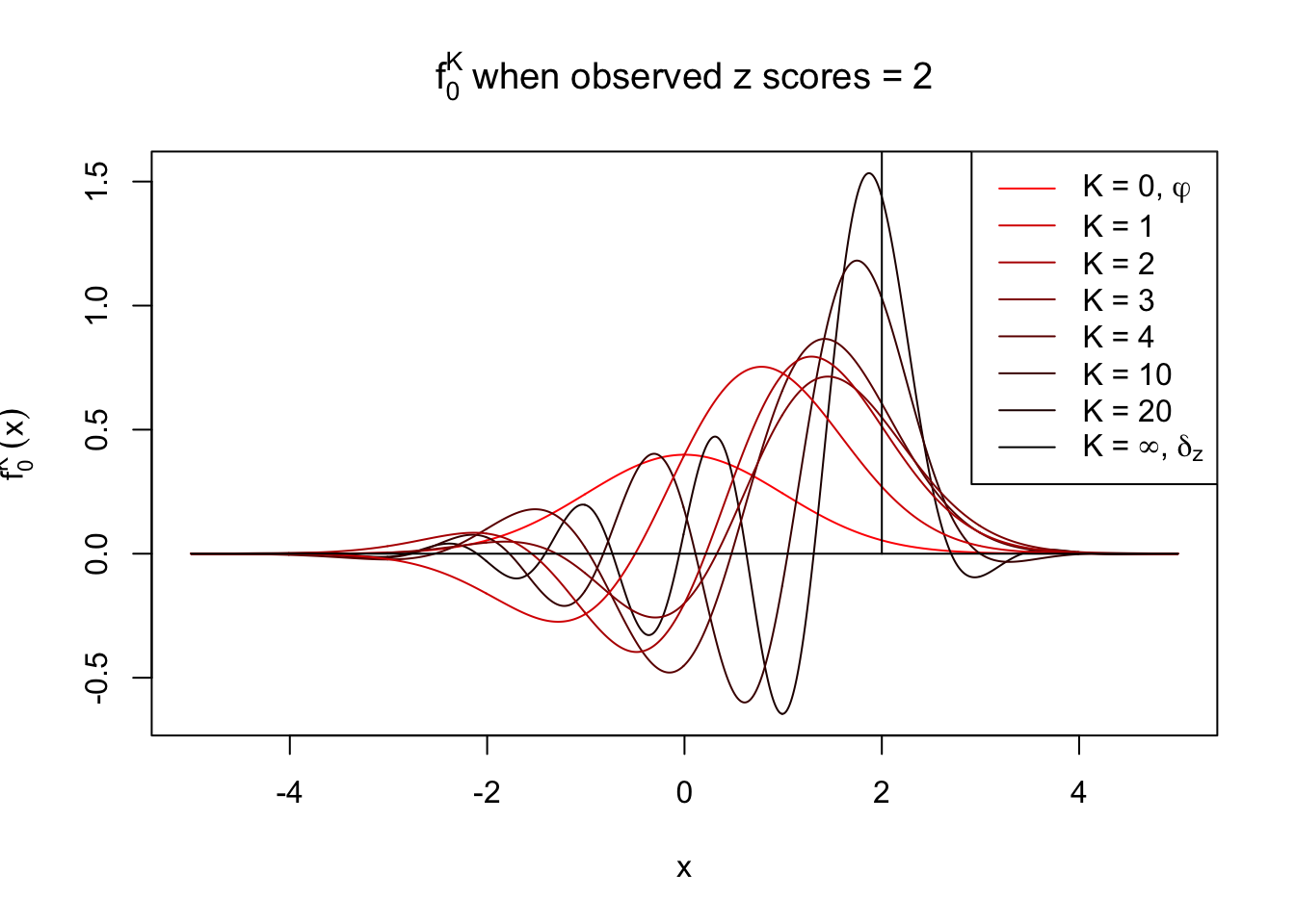
Session information
sessionInfo()R version 3.3.2 (2016-10-31)
Platform: x86_64-apple-darwin13.4.0 (64-bit)
Running under: macOS Sierra 10.12.3
locale:
[1] en_US.UTF-8/en_US.UTF-8/en_US.UTF-8/C/en_US.UTF-8/en_US.UTF-8
attached base packages:
[1] stats graphics grDevices utils datasets methods base
loaded via a namespace (and not attached):
[1] backports_1.0.5 magrittr_1.5 rprojroot_1.2 tools_3.3.2
[5] htmltools_0.3.5 yaml_2.1.14 Rcpp_0.12.10 stringi_1.1.2
[9] rmarkdown_1.3 knitr_1.15.1 stringr_1.2.0 digest_0.6.11
[13] evaluate_0.10 This R Markdown site was created with workflowr