Step-Down Multiple Comparison Procedures on Simulated Correlated Null to Control FWER

Holm-Bonferroni’s procedure

First, order the \(p\)-values

\[ p_{(1)} \leq p_{(2)} \leq \cdots \leq p_{(n)} \]

and let \(H_{(1)}, H_{(2)}, \ldots, H_{(n)}\) be the corresponding hypotheses. Then examine the \(p\)-values in order.

Step 1: If \(p_{(1)} \leq \alpha/n\) reject \(H_{(1)}\) and go to Step 2. Otherwise, accept \(H_{(1)}, H_{(2)}, \ldots, H_{(n)}\) and stop.

Step \(i\): If \(p_{(i)} \leq \alpha / (n − i + 1)\) reject \(H_{(i)}\) and go to step \(i + 1\). Otherwise, accept \(H_{(i)}, H_{(i + 1)}, \ldots, H_{(n)}\) and stop.

Step \(n\): If \(p_{(n)} \leq \alpha\), reject \(H_{(n)}\). Otherwise, accept \(H_{(n)}\).

Hence the procedure starts with the most extreme (smallest) \(p\)-value and stops the first time \(p_{(i)}\) exceeds the critical value \(\alpha_i = \alpha/(n − i + 1)\).

It can be shown that Holm’s procedure controls the FWER strongly, under arbitrary correlation among \(p\)-values.

Sidak-Holm’s procedure

Similar to Holm-Bonferroni’s, only to replace thresholds \(\alpha/n, \alpha/(n-1), \ldots, \alpha\) with \(1 - (1 - \alpha)^{1/n}, 1 - (1 - \alpha)^{1/(n-1)}, \ldots, 1 - (1 - \alpha)^{1}\). Sidak-Holm is more powerful than Holm-Bonferroni; however, it controls FWER only when \(p\)-values are independent. Although we certainly don’t have independent \(p\)-values, nevertheless we hope to see if Sidak-Holm can control FWER for our simulated data.

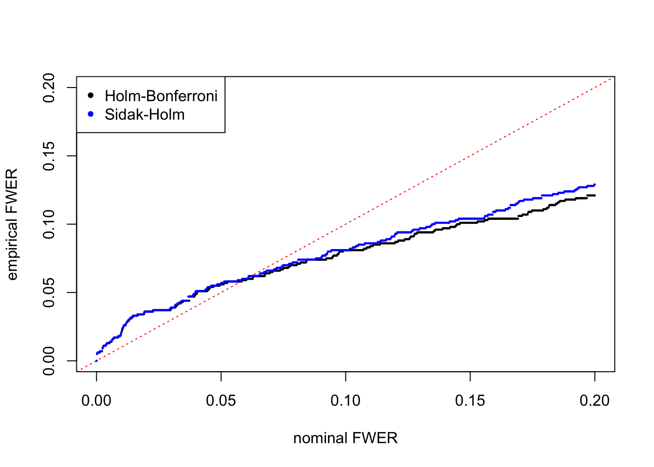
The theoretical result tells us that Holm-Bonferroni controls FWER under any circumstances (arbitrary correlation) whereas Sidak-Holm is guaranteed to control FWER only when p-values are independent. On the other hand, both procedures control FWER very conservatively; that is, under respective assumptions, both procedures are guaranteed to have FWER \(< \alpha\), not \(= \alpha\).

Result

holm = read.table("../output/p_null_liver_holm.txt")
sidak = read.table("../output/p_null_liver_sidak.txt")
alpha = seq(0, 0.2, length = 1000)
fwer_holm = fwer_sidak = c()
for (i in 1:length(alpha)) {
  fwer_holm[i] = mean(apply(holm, 1, function(x) {min(x) <= alpha[i]}))
  fwer_sidak[i] = mean(apply(sidak, 1, function(x) {min(x) <= alpha[i]}))
}

plot(alpha, fwer_holm, pch = 20, xlab = "nominal FWER", ylab = "empirical FWER", xlim = c(0, max(alpha)), ylim = c(0, max(alpha)), cex = 0.25)
abline(0, 1, lty = 3, col = "red")
points(alpha, fwer_sidak, col = "blue", pch = 20, cex = 0.25)
legend("topleft", c("Holm-Bonferroni", "Sidak-Holm"), col = c(1, "blue"), pch = 20)

When \(\alpha > 0.10\), we can see that empirical FWER \(<\) nominal FWER, even though we would have inflated (not so extreme) \(p\)-values coming into play, suggesting a certain level of conservativeness. When \(\alpha\) is small, though, we do see in this simulation run empirical FWER \(>\) nominal FWER, but I would argue that it’s actually not that big. For example, when nominal FWER \(= 0.05\), empirical FWER of Holm_Bonferroni is \(0.056\) and that of Sidak-Holm is \(0.057\), fairly close to \(0.05\). Second, simulations with smaller \(\alpha\) might be more prone to randomness in the simulation.

Here is another simulation, with only the random seed changed from \(101\) to \(1\) but nothing else.

Another simulation run with a different random seed

This simulation only change the random seed from \(101\) to \(1\) but nothing else, and empirical FWER for both procedures looks much better. I’m thinking it shows that VOOM does give \(p\)-values marginally uniform under the global null, and starting with most extreme \(p\)-values for correlated null data could control FWER.

The code to generate adjusted \(p\)-values are stored in StepDown.R

Session Information

sessionInfo()

R version 3.3.2 (2016-10-31)
Platform: x86_64-apple-darwin13.4.0 (64-bit)
Running under: macOS Sierra 10.12.3

locale:
[1] en_US.UTF-8/en_US.UTF-8/en_US.UTF-8/C/en_US.UTF-8/en_US.UTF-8

attached base packages:
[1] stats     graphics  grDevices utils     datasets  methods   base     

other attached packages:
[1] workflowr_0.3.0 rmarkdown_1.3  

loaded via a namespace (and not attached):
 [1] backports_1.0.5  magrittr_1.5     rprojroot_1.2    htmltools_0.3.5 
 [5] tools_3.3.2      yaml_2.1.14      Rcpp_0.12.9      codetools_0.2-15
 [9] stringi_1.1.2    knitr_1.15.1     git2r_0.18.0     stringr_1.1.0   
[13] digest_0.6.11    evaluate_0.10