Poisson to approximate binomial
Dongyue Xie
May 15, 2018
Last updated: 2018-05-18
workflowr checks: (Click a bullet for more information)-
✔ R Markdown file: up-to-date
Great! Since the R Markdown file has been committed to the Git repository, you know the exact version of the code that produced these results.
-
✔ Environment: empty
Great job! The global environment was empty. Objects defined in the global environment can affect the analysis in your R Markdown file in unknown ways. For reproduciblity it’s best to always run the code in an empty environment.
-
✔ Seed:
set.seed(20180501)The command
set.seed(20180501)was run prior to running the code in the R Markdown file. Setting a seed ensures that any results that rely on randomness, e.g. subsampling or permutations, are reproducible. -
✔ Session information: recorded
Great job! Recording the operating system, R version, and package versions is critical for reproducibility.
-
Great! You are using Git for version control. Tracking code development and connecting the code version to the results is critical for reproducibility. The version displayed above was the version of the Git repository at the time these results were generated.✔ Repository version: 585d9b1
Note that you need to be careful to ensure that all relevant files for the analysis have been committed to Git prior to generating the results (you can usewflow_publishorwflow_git_commit). workflowr only checks the R Markdown file, but you know if there are other scripts or data files that it depends on. Below is the status of the Git repository when the results were generated:
Note that any generated files, e.g. HTML, png, CSS, etc., are not included in this status report because it is ok for generated content to have uncommitted changes.Ignored files: Ignored: .Rhistory Ignored: .Rproj.user/ Ignored: log/ Untracked files: Untracked: analysis/binom.Rmd Untracked: analysis/overdis.Rmd Untracked: analysis/smashtutorial.Rmd Untracked: data/treas_bill.csv Untracked: docs/figure/smashtutorial.Rmd/ Unstaged changes: Modified: analysis/ashpmean.Rmd Modified: analysis/nugget.Rmd
Expand here to see past versions:
| File | Version | Author | Date | Message |
|---|---|---|---|---|
| Rmd | 585d9b1 | Dongyue | 2018-05-18 | binomial smooth vs poibinom |
Methods
Let \(X\sim Binomial(n,p)\) then \(E(X)=np, Var(X)=np(1-p)\). Poisson distribution is an approximation of binomial distribution when \(n\) is large and \(p\) is small. A rule of thumb is that \(n\geq 20, p\leq 0.05\).
Derivation: Let \(\lambda=np\)
\[\frac{n!}{x!(n-x)!}p^x(1-p)^{n-x}=\frac{n(n-1)...(n-k+1)}{x!}(\lambda/n)^x(1-\lambda/n)^{n-x}\approx \frac{\lambda^x}{x!}(1-\lambda/n)^{n-x}\] as \(n\to \infty\). Since \(lim_{n\to \infty}(1-\lambda/n)^{n}=e^{-\lambda}\) and \(lim_{n\to \infty}(1-\lambda/n)^{-x}=1\), we have \[\frac{n!}{x!(n-x)!}p^x(1-p)^{n-x}\approx \frac{\lambda^x e^{-\lambda}}{x!}.\]
If we have binomial observation \(X_t\) with \(n_t\) and treat it as Poisson observation, we can do the following expansion: \[Y_t=\log(X_t)=\log(n_tp_t)+\frac{X_t-n_tp_t}{n_tp_t}=\log(n_t)+\log(p_t)+\frac{X_t-n_tp_t}{n_tp_t}.\] This leads to \[Y_t-\log(n_t)=\log(p_t)+\frac{X_t-n_tp_t}{n_tp_t}.\]
Experiments
We compare the performance of smashgen - binomial and smashgen - poi_binom, as well as Translation Invariant (TI) thresholding (Coifman and Donoho, 1995), which is one of the best methods in a large-scale simulation study in Antoniadis et al. (2001), and Ebayesthresh (Johnstone and Silverman, 2005b).
For all experiments, T is set to be 256, nugget effect \(\sigma=1\). The mean squared errors are reported and the plots are served as visual aids.
library(smashrgen)
library(ggplot2)
library(EbayesThresh)

simu_study=function(p,sigma=1,ntri,nsimu=100,seed=12345,
                    niter=1,family='DaubExPhase',ashp=TRUE,verbose=FALSE,robust=FALSE,
                    tol=1e-2){
  set.seed(seed)
  smash.binom.err=c()
  smash.poibinom.err=c()
  ti.thresh.err=c()
  eb.thresh.err=c()
  n=length(p)
  target=exp(p)/(1+exp(p))
  for(k in 1:nsimu){
    ng=rnorm(n,0,sigma)
    m=exp(p+ng)
    q=m/(1+m)
    x=rbinom(n,ntri,q)
    #fit data
    smash.binom.out=smash_gen(x,dist_family = 'binomial',y_var_est='smashu',ntri=ntri)
    smash.poibinom.out=smash_gen(x,dist_family = 'poi_binom',y_var_est='smashu',ntri=ntri)
    ti.thresh.out=ti.thresh(x/ntri,method='rmad')
    eb.thresh.out=waveti.ebayes(x/ntri)
    #errors
    smash.binom.err[k]=mse(target,smash.binom.out)
    smash.poibinom.err[k]=mse(target,smash.poibinom.out)
    ti.thresh.err[k]=mse(target,ti.thresh.out)
    eb.thresh.err[k]=mse(target,eb.thresh.out)
  }
  return(list(est=list(smash.binom.out=smash.binom.out,smash.poibinom.out=smash.poibinom.out, ti.thresh.out=ti.thresh.out,eb.thresh.out=eb.thresh.out,x=x),
              err=data.frame(smash.binom=smash.binom.err,smash.poibinom=smash.poibinom.err, ti.thresh=ti.thresh.err,eb.thresh=eb.thresh.err)))
}

waveti.ebayes = function(x, filter.number = 10, family = "DaubLeAsymm", min.level = 3) {
    n = length(x)
    J = log2(n)
    x.w = wd(x, filter.number, family, type = "station")
    for (j in min.level:(J - 1)) {
        x.pm = ebayesthresh(accessD(x.w, j))
        x.w = putD(x.w, j, x.pm)
    }
    mu.est = AvBasis(convert(x.w))
    return(mu.est)
}
Constant trend
\(ntri\) large, \(p\) large
The number of trials are generated from a Poisson distribution with \(\lambda=50\). \(p\) is around 0.8.
n=256
p=rep(1.5,n)
set.seed(111)
ntri=rpois(n,50)
result=simu_study(p,ntri=ntri)

ggplot(df2gg(result$err),aes(x=method,y=MSE))+geom_boxplot(aes(fill=method))+labs(x='')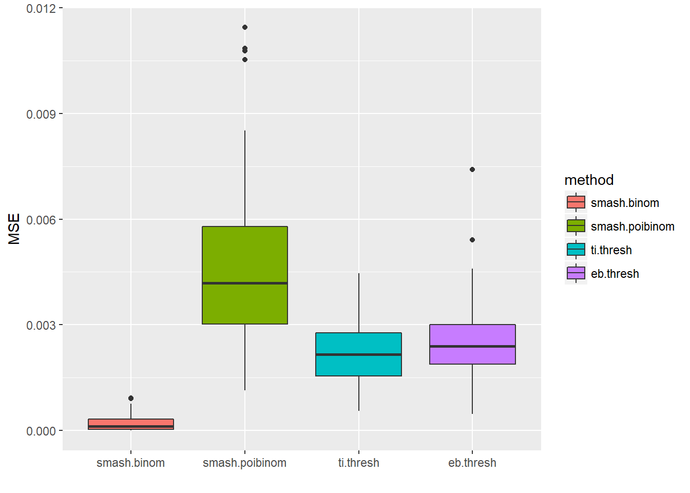
par(mfrow=c(2,2))
plot(result$est$x/ntri,col='gray80',ylab='',main='smash-binom')
lines(exp(p)/(1+exp(p)),lty=2)
lines(result$est$smash.binom.out,col=4,lwd=2)
legend("bottomright", # places a legend at the appropriate place
       c("truth","smash-binom"), # puts text in the legend
       lty=c(2,1), # gives the legend appropriate symbols (lines)
       lwd=c(1,2),
       cex = 1,
       col=c("black","blue"))
plot(result$est$x/ntri,col='gray80',ylab='',main='smash-poi_binom')
lines(exp(p)/(1+exp(p)),lty=2)
lines(result$est$smash.poibinom.out,col=4,lwd=2)
plot(result$est$x/ntri,col='gray80',ylab='',main='TI thresh')
lines(exp(p)/(1+exp(p)),lty=2)
lines(result$est$ti.thresh.out,col=4,lwd=2)
plot(result$est$x/ntri,col='gray80',ylab='',main='EBayes thresh')
lines(exp(p)/(1+exp(p)),lty=2)
lines(result$est$eb.thresh.out,col=4,lwd=2)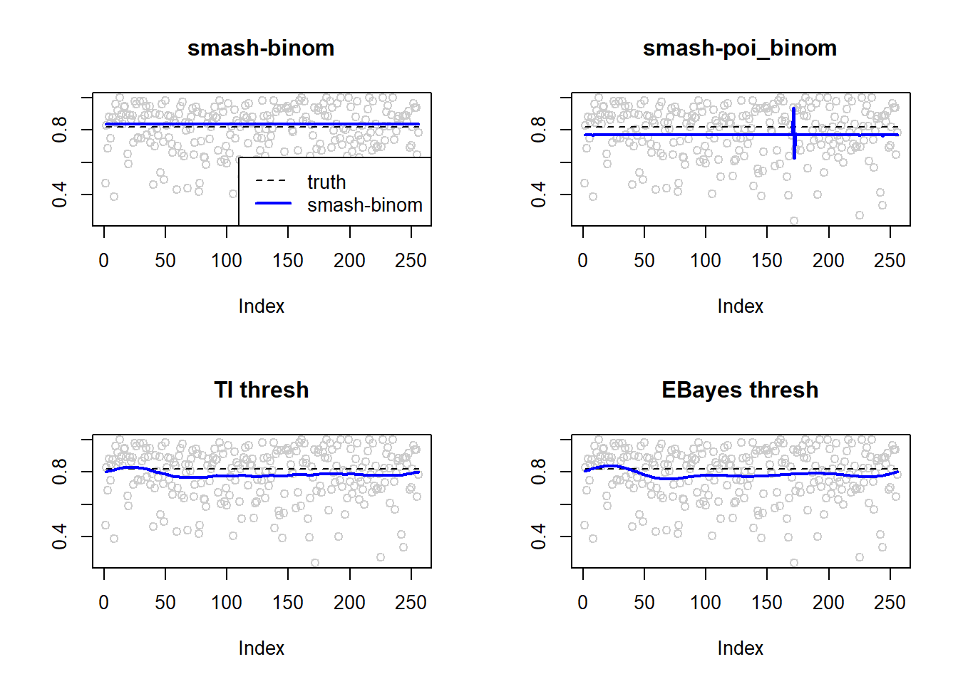
\(ntri\) small, \(p\) large
The number of trials are generated from a Poisson distribution with \(\lambda=8\). \(p\) is around 0.8.
n=256
p=rep(1.5,n)
set.seed(111)
ntri=rpois(n,5)+1
result=simu_study(p,ntri=ntri)

ggplot(df2gg(result$err),aes(x=method,y=MSE))+geom_boxplot(aes(fill=method))+labs(x='')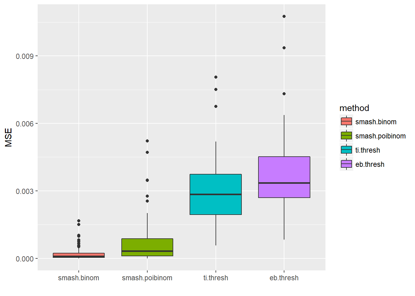
par(mfrow=c(2,2))
plot(result$est$x/ntri,col='gray80',ylab='',main='smash-binom')
lines(exp(p)/(1+exp(p)),lty=2)
lines(result$est$smash.binom.out,col=4,lwd=2)
legend("bottomright", # places a legend at the appropriate place
       c("truth","smash-binom"), # puts text in the legend
       lty=c(2,1), # gives the legend appropriate symbols (lines)
       lwd=c(1,2),
       cex = 1,
       col=c("black","blue"))
plot(result$est$x/ntri,col='gray80',ylab='',main='smash-poi_binom')
lines(exp(p)/(1+exp(p)),lty=2)
lines(result$est$smash.poibinom.out,col=4,lwd=2)
plot(result$est$x/ntri,col='gray80',ylab='',main='TI thresh')
lines(exp(p)/(1+exp(p)),lty=2)
lines(result$est$ti.thresh.out,col=4,lwd=2)
plot(result$est$x/ntri,col='gray80',ylab='',main='EBayes thresh')
lines(exp(p)/(1+exp(p)),lty=2)
lines(result$est$eb.thresh.out,col=4,lwd=2)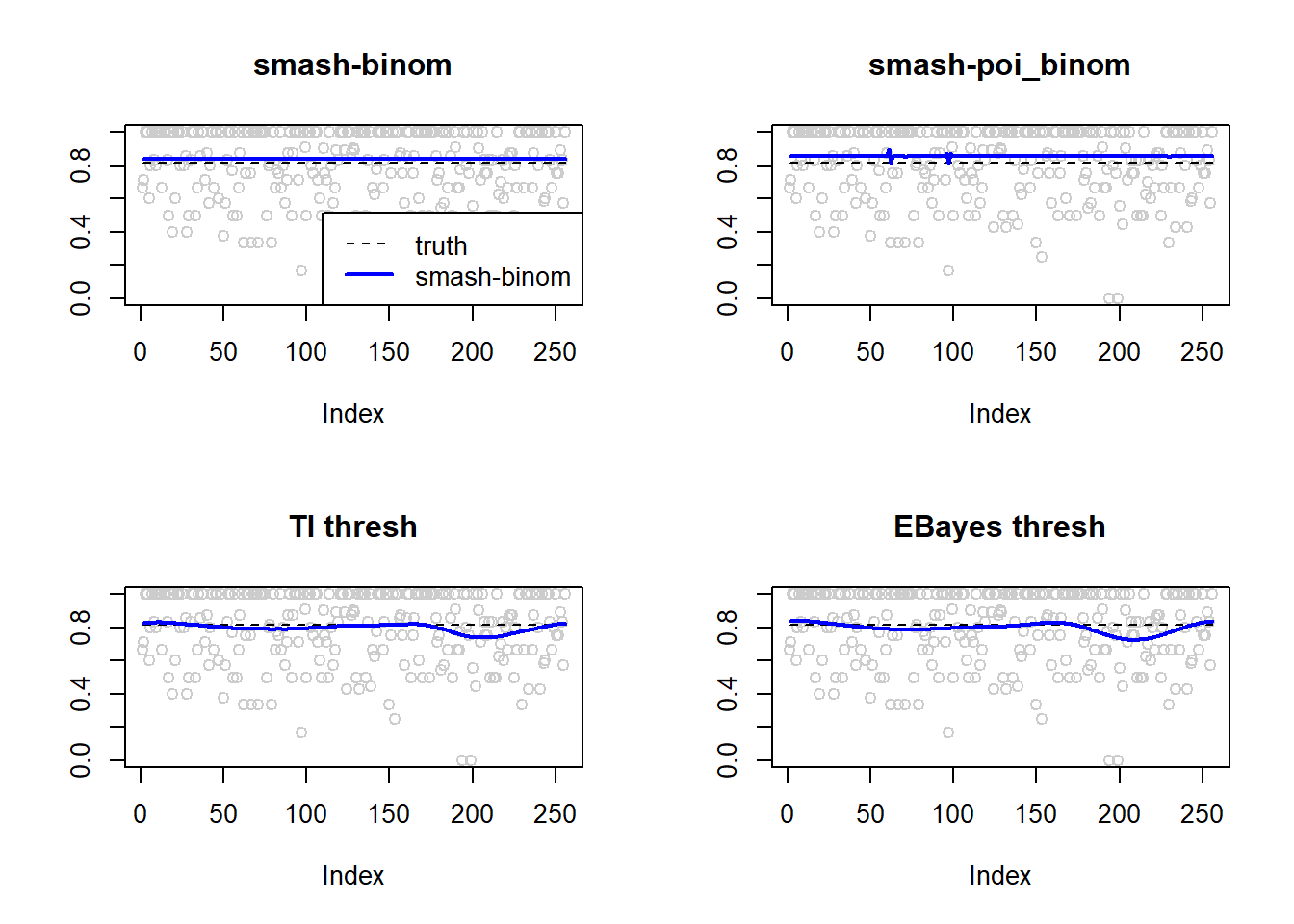
\(ntri\) large, \(p\) small
The number of trials are generated from a Poisson distribution with \(\lambda=50\). \(p\) is around 0.05.
n=256
p=rep(-3,n)
set.seed(111)
ntri=rpois(n,50)
result=simu_study(p,ntri=ntri)

ggplot(df2gg(result$err),aes(x=method,y=MSE))+geom_boxplot(aes(fill=method))+labs(x='')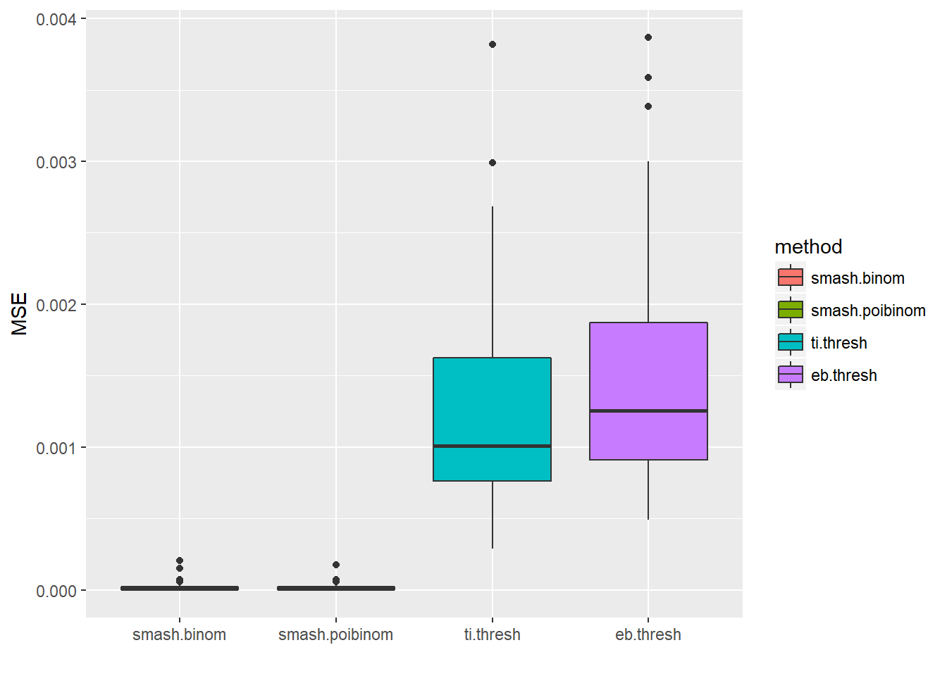
ggplot(df2gg(result$err[,1:2]),aes(x=method,y=MSE))+geom_boxplot(aes(fill=method))+labs(x='')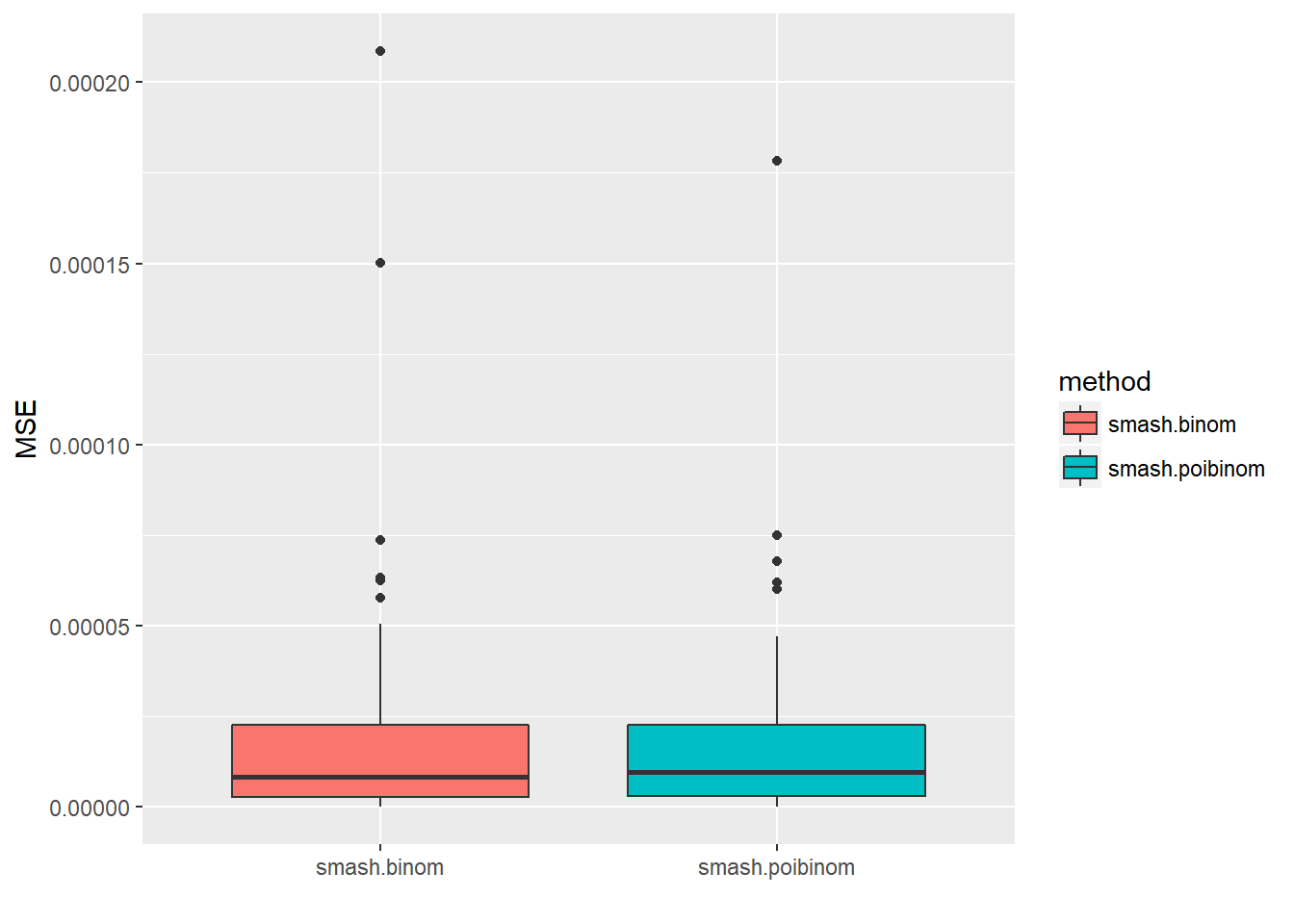
par(mfrow=c(2,2))
plot(result$est$x/ntri,col='gray80',ylab='',main='smash-binom')
lines(exp(p)/(1+exp(p)),lty=2)
lines(result$est$smash.binom.out,col=4,lwd=2)
legend("bottomright", # places a legend at the appropriate place
       c("truth","smash-binom"), # puts text in the legend
       lty=c(2,1), # gives the legend appropriate symbols (lines)
       lwd=c(1,2),
       cex = 1,
       col=c("black","blue"))
plot(result$est$x/ntri,col='gray80',ylab='',main='smash-poi_binom')
lines(exp(p)/(1+exp(p)),lty=2)
lines(result$est$smash.poibinom.out,col=4,lwd=2)
plot(result$est$x/ntri,col='gray80',ylab='',main='TI thresh')
lines(exp(p)/(1+exp(p)),lty=2)
lines(result$est$ti.thresh.out,col=4,lwd=2)
plot(result$est$x/ntri,col='gray80',ylab='',main='EBayes thresh')
lines(exp(p)/(1+exp(p)),lty=2)
lines(result$est$eb.thresh.out,col=4,lwd=2)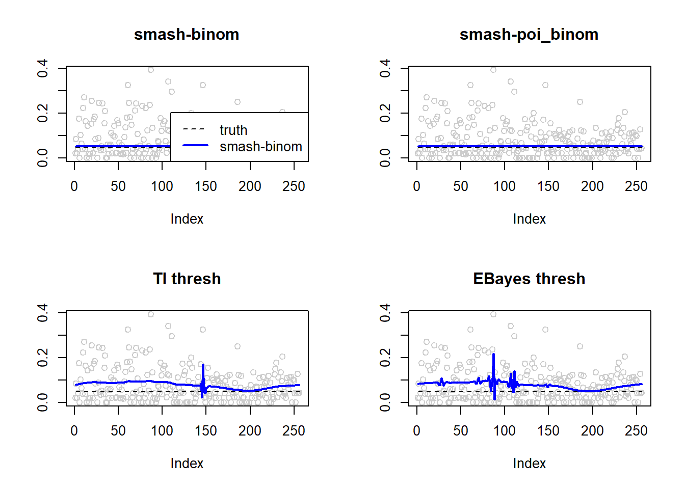
As expected, when \(n\) is large and \(p\) is small, Poisson distribution is a good approximation to binomial distribution.
\(ntri\) small, \(p\) small
The number of trials are generated from a Poisson distribution with \(\lambda=5\). \(p\) is around 0.05.
n=256
p=rep(-3,n)
set.seed(111)
ntri=rpois(n,5)+1
result=simu_study(p,ntri=ntri)

ggplot(df2gg(result$err),aes(x=method,y=MSE))+geom_boxplot(aes(fill=method))+labs(x='')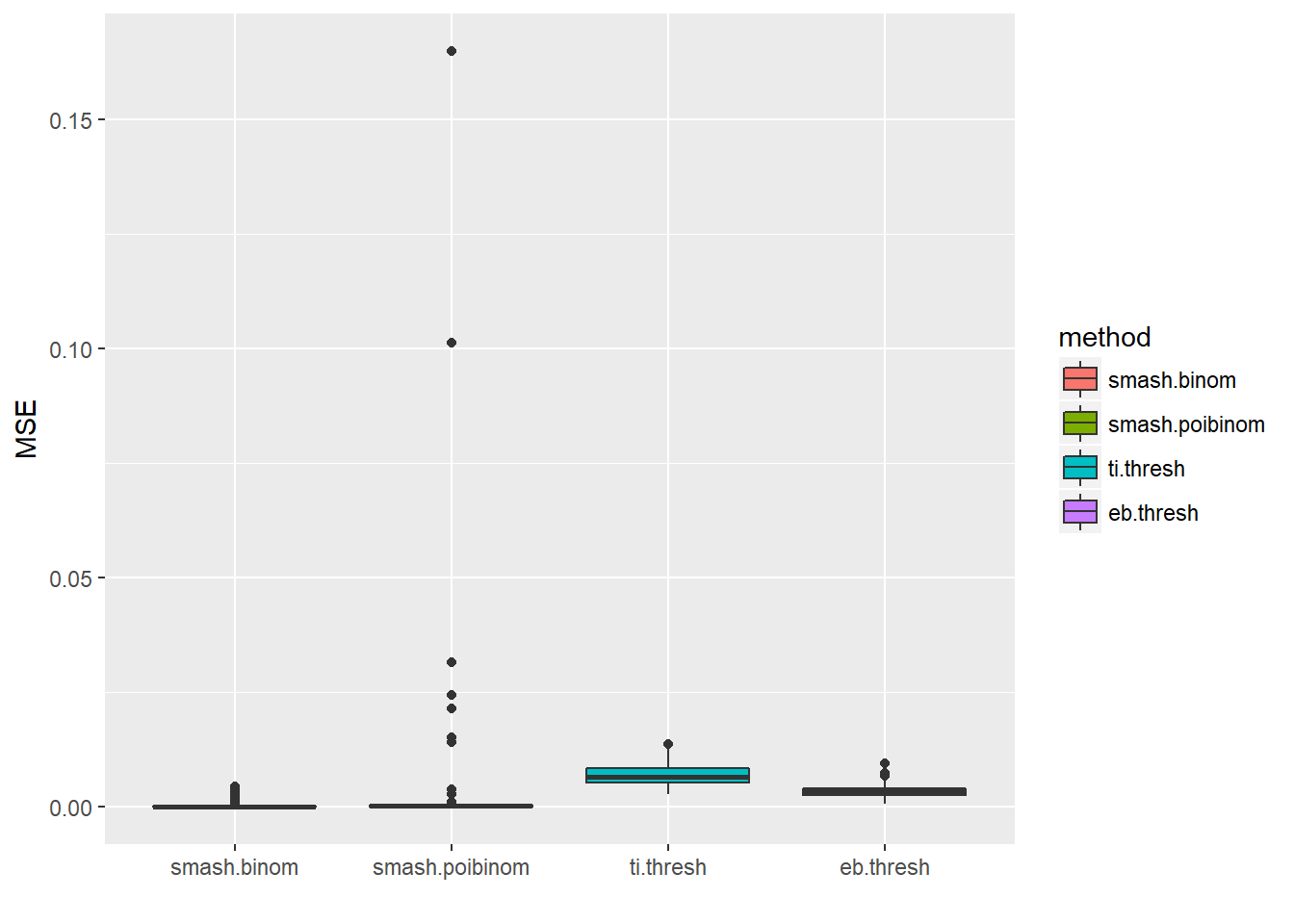
par(mfrow=c(2,2))
plot(result$est$x/ntri,col='gray80',ylab='',main='smash-binom')
lines(exp(p)/(1+exp(p)),lty=2)
lines(result$est$smash.binom.out,col=4,lwd=2)
legend("bottomright", # places a legend at the appropriate place
       c("truth","smash-binom"), # puts text in the legend
       lty=c(2,1), # gives the legend appropriate symbols (lines)
       lwd=c(1,2),
       cex = 1,
       col=c("black","blue"))
plot(result$est$x/ntri,col='gray80',ylab='',main='smash-poi_binom')
lines(exp(p)/(1+exp(p)),lty=2)
lines(result$est$smash.poibinom.out,col=4,lwd=2)
plot(result$est$x/ntri,col='gray80',ylab='',main='TI thresh')
lines(exp(p)/(1+exp(p)),lty=2)
lines(result$est$ti.thresh.out,col=4,lwd=2)
plot(result$est$x/ntri,col='gray80',ylab='',main='EBayes thresh')
lines(exp(p)/(1+exp(p)),lty=2)
lines(result$est$eb.thresh.out,col=4,lwd=2)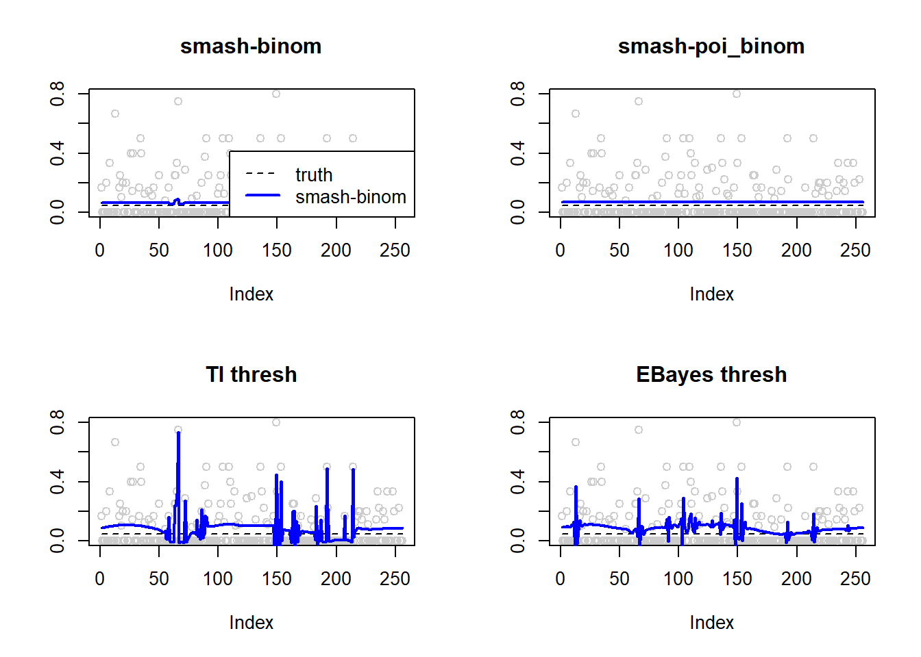
Steps
Large \(n\)
p=c(rep(-2,64), rep(0, 64), rep(2, 64), rep(-2, 64))
set.seed(111)
ntri=rpois(256,50)
result=simu_study(p,ntri=ntri)

ggplot(df2gg(result$err),aes(x=method,y=MSE))+geom_boxplot(aes(fill=method))+labs(x='')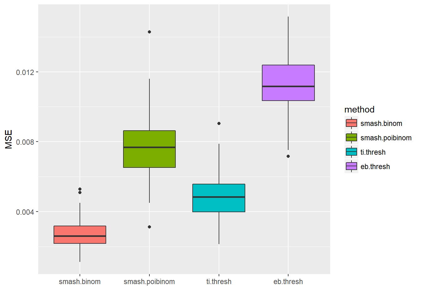
par(mfrow=c(2,2))
plot(result$est$x/ntri,col='gray80',ylab='',main='smash-binom')
lines(exp(p)/(1+exp(p)),lty=2)
lines(result$est$smash.binom.out,col=4,lwd=2)
legend("bottomright", # places a legend at the appropriate place
       c("truth","smash-binom"), # puts text in the legend
       lty=c(2,1), # gives the legend appropriate symbols (lines)
       lwd=c(1,2),
       cex = 1,
       col=c("black","blue"))
plot(result$est$x/ntri,col='gray80',ylab='',main='smash-poi_binom')
lines(exp(p)/(1+exp(p)),lty=2)
lines(result$est$smash.poibinom.out,col=4,lwd=2)
plot(result$est$x/ntri,col='gray80',ylab='',main='TI thresh')
lines(exp(p)/(1+exp(p)),lty=2)
lines(result$est$ti.thresh.out,col=4,lwd=2)
plot(result$est$x/ntri,col='gray80',ylab='',main='EBayes thresh')
lines(exp(p)/(1+exp(p)),lty=2)
lines(result$est$eb.thresh.out,col=4,lwd=2)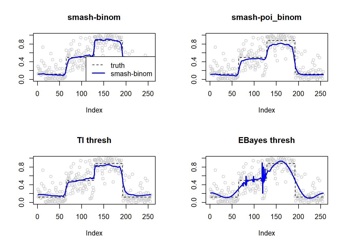
Small \(n\)
p=c(rep(-2,64), rep(0, 64), rep(2, 64), rep(-2, 64))
set.seed(111)
ntri=rpois(256,5)+1
result=simu_study(p,ntri=ntri)

ggplot(df2gg(result$err),aes(x=method,y=MSE))+geom_boxplot(aes(fill=method))+labs(x='')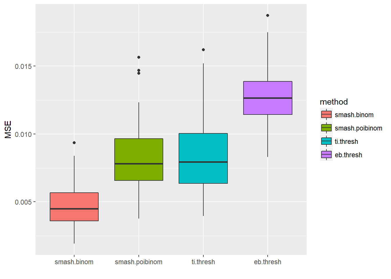
par(mfrow=c(2,2))
plot(result$est$x/ntri,col='gray80',ylab='',main='smash-binom')
lines(exp(p)/(1+exp(p)),lty=2)
lines(result$est$smash.binom.out,col=4,lwd=2)
legend("bottomright", # places a legend at the appropriate place
       c("truth","smash-binom"), # puts text in the legend
       lty=c(2,1), # gives the legend appropriate symbols (lines)
       lwd=c(1,2),
       cex = 1,
       col=c("black","blue"))
plot(result$est$x/ntri,col='gray80',ylab='',main='smash-poi_binom')
lines(exp(p)/(1+exp(p)),lty=2)
lines(result$est$smash.poibinom.out,col=4,lwd=2)
plot(result$est$x/ntri,col='gray80',ylab='',main='TI thresh')
lines(exp(p)/(1+exp(p)),lty=2)
lines(result$est$ti.thresh.out,col=4,lwd=2)
plot(result$est$x/ntri,col='gray80',ylab='',main='EBayes thresh')
lines(exp(p)/(1+exp(p)),lty=2)
lines(result$est$eb.thresh.out,col=4,lwd=2)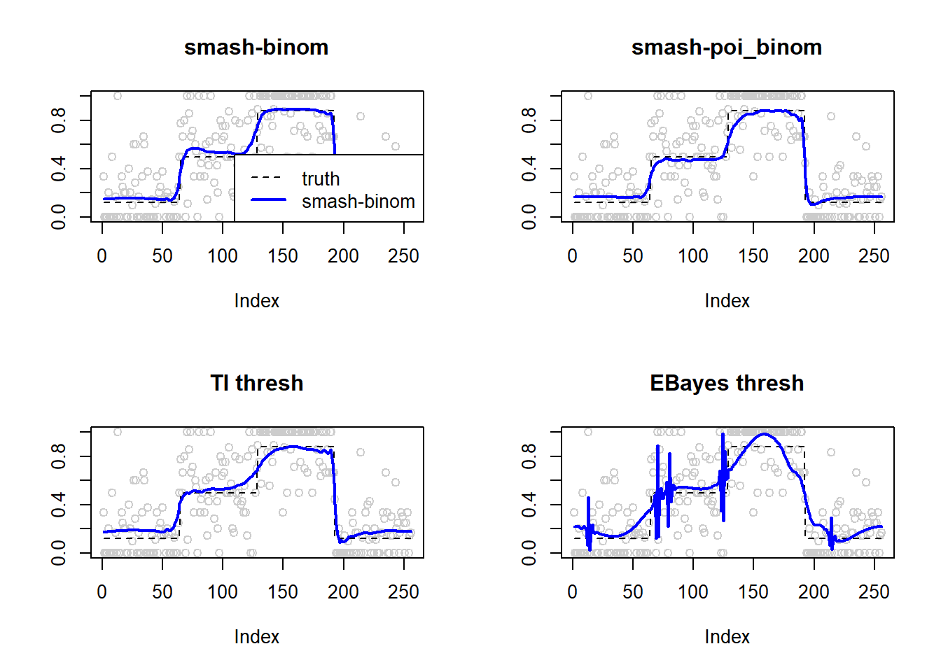
Bumps
Large \(n\).
m=seq(0,1,length.out = 256)
h = c(4, 5, 3, 4, 5, 4.2, 2.1, 4.3, 3.1, 5.1, 4.2)
w = c(0.005, 0.005, 0.006, 0.01, 0.01, 0.03, 0.01, 0.01, 0.005,0.008,0.005)
t=c(.1,.13,.15,.23,.25,.4,.44,.65,.76,.78,.81)
f = c()
for(i in 1:length(m)){
  f[i]=sum(h*(1+((m[i]-t)/w)^4)^(-1))
}
p=f-3

set.seed(111)
ntri=rpois(256,50)
result=simu_study(p,ntri=ntri)

ggplot(df2gg(result$err),aes(x=method,y=MSE))+geom_boxplot(aes(fill=method))+labs(x='')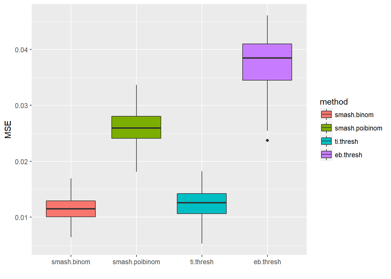
par(mfrow=c(2,2))
plot(result$est$x/ntri,col='gray80',ylab='',main='smash-binom')
lines(exp(p)/(1+exp(p)),lty=2)
lines(result$est$smash.binom.out,col=4,lwd=2)
legend("bottomright", # places a legend at the appropriate place
       c("truth","smash-binom"), # puts text in the legend
       lty=c(2,1), # gives the legend appropriate symbols (lines)
       lwd=c(1,2),
       cex = 1,
       col=c("black","blue"))
plot(result$est$x/ntri,col='gray80',ylab='',main='smash-poi_binom')
lines(exp(p)/(1+exp(p)),lty=2)
lines(result$est$smash.poibinom.out,col=4,lwd=2)
plot(result$est$x/ntri,col='gray80',ylab='',main='TI thresh')
lines(exp(p)/(1+exp(p)),lty=2)
lines(result$est$ti.thresh.out,col=4,lwd=2)
plot(result$est$x/ntri,col='gray80',ylab='',main='EBayes thresh')
lines(exp(p)/(1+exp(p)),lty=2)
lines(result$est$eb.thresh.out,col=4,lwd=2)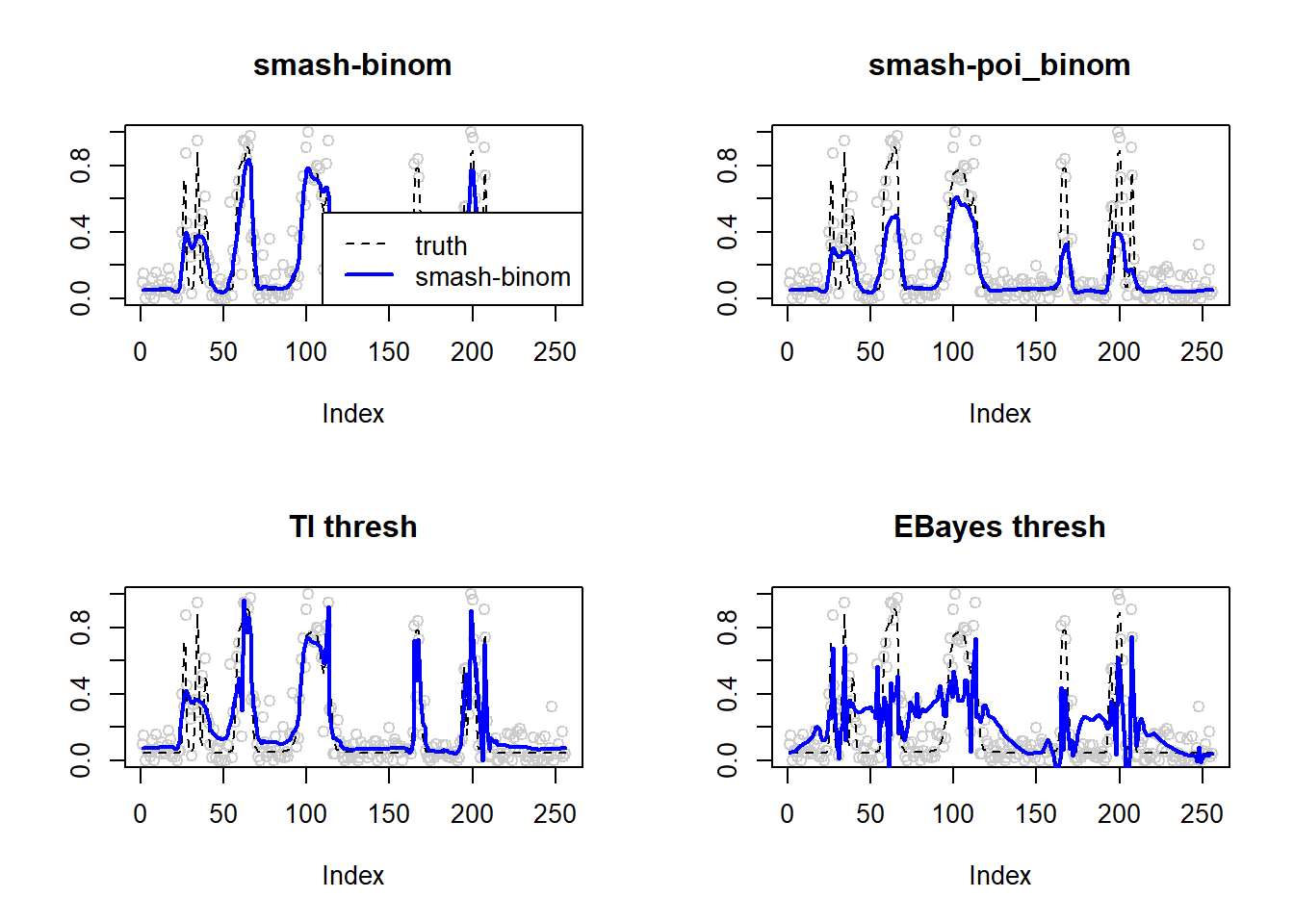
Small \(n\)
set.seed(111)
ntri=rpois(256,5)+1
result=simu_study(p,ntri=ntri)

ggplot(df2gg(result$err),aes(x=method,y=MSE))+geom_boxplot(aes(fill=method))+labs(x='')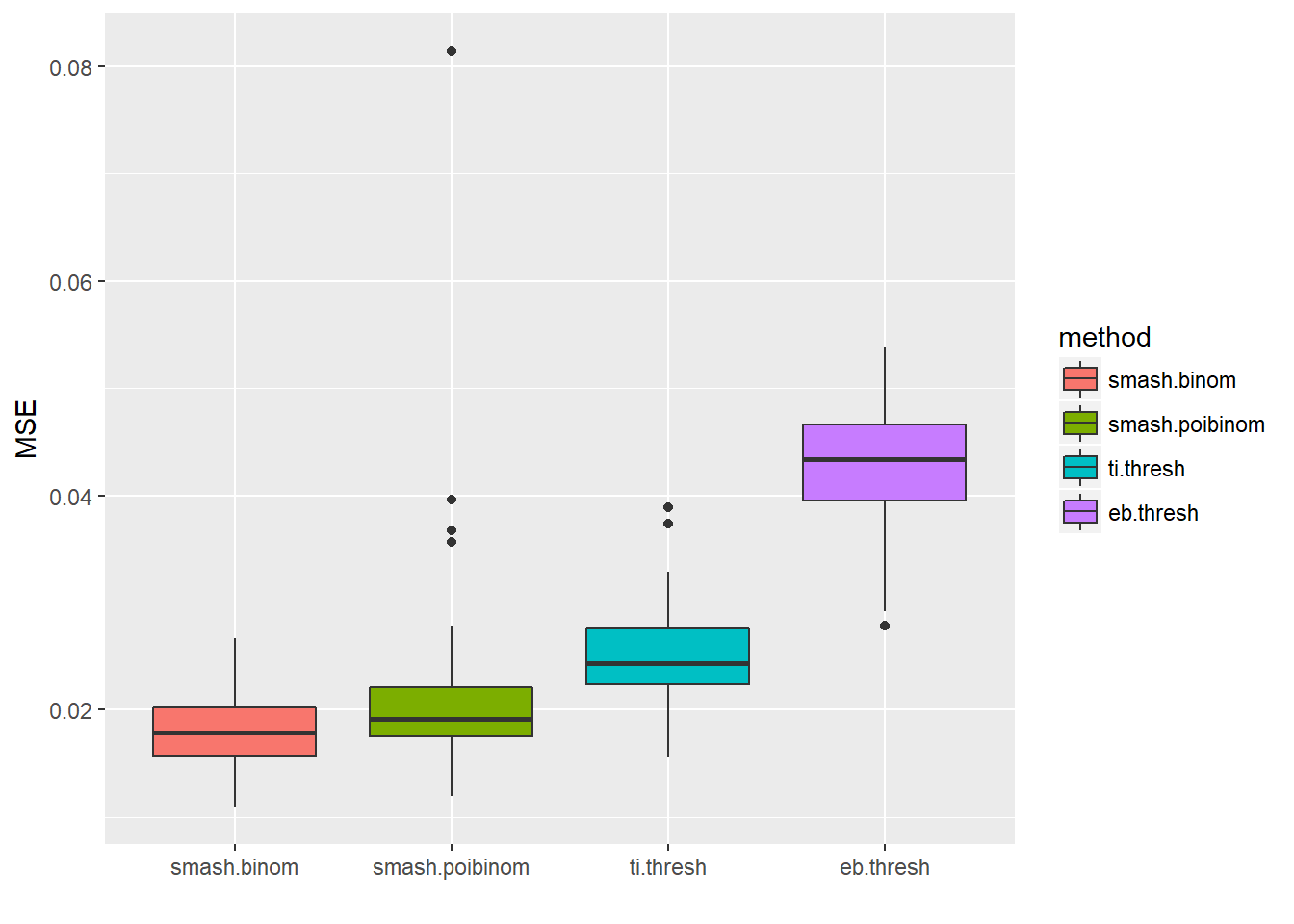
par(mfrow=c(2,2))
plot(result$est$x/ntri,col='gray80',ylab='',main='smash-binom')
lines(exp(p)/(1+exp(p)),lty=2)
lines(result$est$smash.binom.out,col=4,lwd=2)
legend("bottomright", # places a legend at the appropriate place
       c("truth","smash-binom"), # puts text in the legend
       lty=c(2,1), # gives the legend appropriate symbols (lines)
       lwd=c(1,2),
       cex = 1,
       col=c("black","blue"))
plot(result$est$x/ntri,col='gray80',ylab='',main='smash-poi_binom')
lines(exp(p)/(1+exp(p)),lty=2)
lines(result$est$smash.poibinom.out,col=4,lwd=2)
plot(result$est$x/ntri,col='gray80',ylab='',main='TI thresh')
lines(exp(p)/(1+exp(p)),lty=2)
lines(result$est$ti.thresh.out,col=4,lwd=2)
plot(result$est$x/ntri,col='gray80',ylab='',main='EBayes thresh')
lines(exp(p)/(1+exp(p)),lty=2)
lines(result$est$eb.thresh.out,col=4,lwd=2)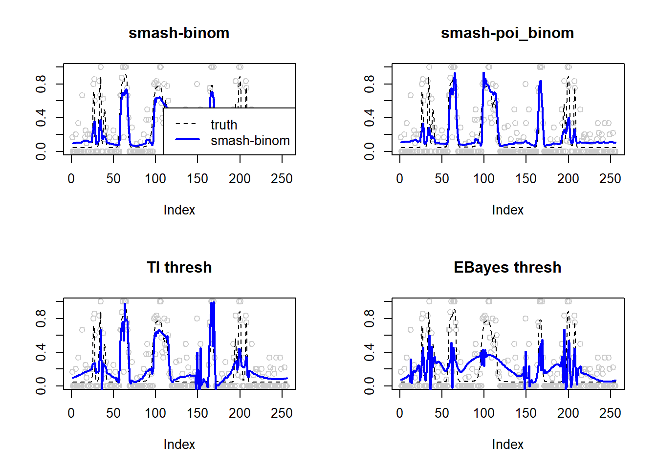
Spike mean
Large \(n\)
spike.f = function(x) (0.75 * exp(-500 * (x - 0.23)^2) + 1.5 * exp(-2000 * (x - 0.33)^2) + 3 * exp(-8000 * (x - 0.47)^2) + 2.25 * exp(-16000 *
    (x - 0.69)^2) + 0.5 * exp(-32000 * (x - 0.83)^2))
n = 256
t = 1:n/n
p = spike.f(t)*2-2

set.seed(111)
ntri=rpois(256,50)
result=simu_study(p,ntri=ntri)

ggplot(df2gg(result$err),aes(x=method,y=MSE))+geom_boxplot(aes(fill=method))+labs(x='')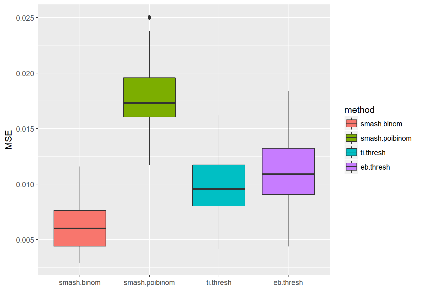
par(mfrow=c(2,2))
plot(result$est$x/ntri,col='gray80',ylab='',main='smash-binom')
lines(exp(p)/(1+exp(p)),lty=2)
lines(result$est$smash.binom.out,col=4,lwd=2)
legend("bottomright", # places a legend at the appropriate place
       c("truth","smash-binom"), # puts text in the legend
       lty=c(2,1), # gives the legend appropriate symbols (lines)
       lwd=c(1,2),
       cex = 1,
       col=c("black","blue"))
plot(result$est$x/ntri,col='gray80',ylab='',main='smash-poi_binom')
lines(exp(p)/(1+exp(p)),lty=2)
lines(result$est$smash.poibinom.out,col=4,lwd=2)
plot(result$est$x/ntri,col='gray80',ylab='',main='TI thresh')
lines(exp(p)/(1+exp(p)),lty=2)
lines(result$est$ti.thresh.out,col=4,lwd=2)
plot(result$est$x/ntri,col='gray80',ylab='',main='EBayes thresh')
lines(exp(p)/(1+exp(p)),lty=2)
lines(result$est$eb.thresh.out,col=4,lwd=2)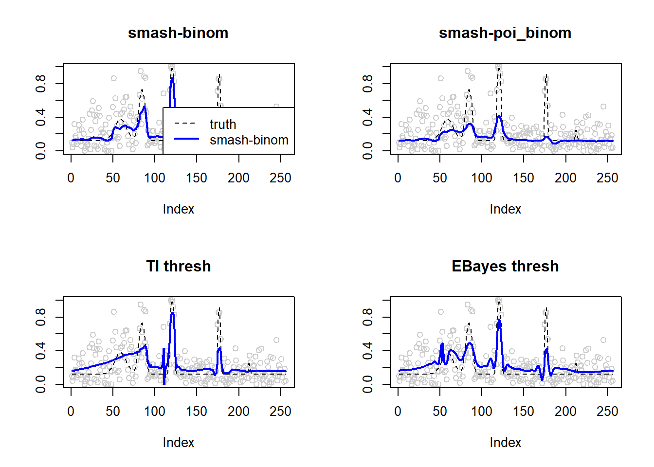
Small \(n\)
set.seed(111)
ntri=rpois(256,5)+1
result=simu_study(p,ntri=ntri)

ggplot(df2gg(result$err),aes(x=method,y=MSE))+geom_boxplot(aes(fill=method))+labs(x='')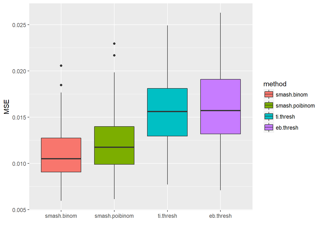
par(mfrow=c(2,2))
plot(result$est$x/ntri,col='gray80',ylab='',main='smash-binom')
lines(exp(p)/(1+exp(p)),lty=2)
lines(result$est$smash.binom.out,col=4,lwd=2)
legend("bottomright", # places a legend at the appropriate place
       c("truth","smash-binom"), # puts text in the legend
       lty=c(2,1), # gives the legend appropriate symbols (lines)
       lwd=c(1,2),
       cex = 1,
       col=c("black","blue"))
plot(result$est$x/ntri,col='gray80',ylab='',main='smash-poi_binom')
lines(exp(p)/(1+exp(p)),lty=2)
lines(result$est$smash.poibinom.out,col=4,lwd=2)
plot(result$est$x/ntri,col='gray80',ylab='',main='TI thresh')
lines(exp(p)/(1+exp(p)),lty=2)
lines(result$est$ti.thresh.out,col=4,lwd=2)
plot(result$est$x/ntri,col='gray80',ylab='',main='EBayes thresh')
lines(exp(p)/(1+exp(p)),lty=2)
lines(result$est$eb.thresh.out,col=4,lwd=2)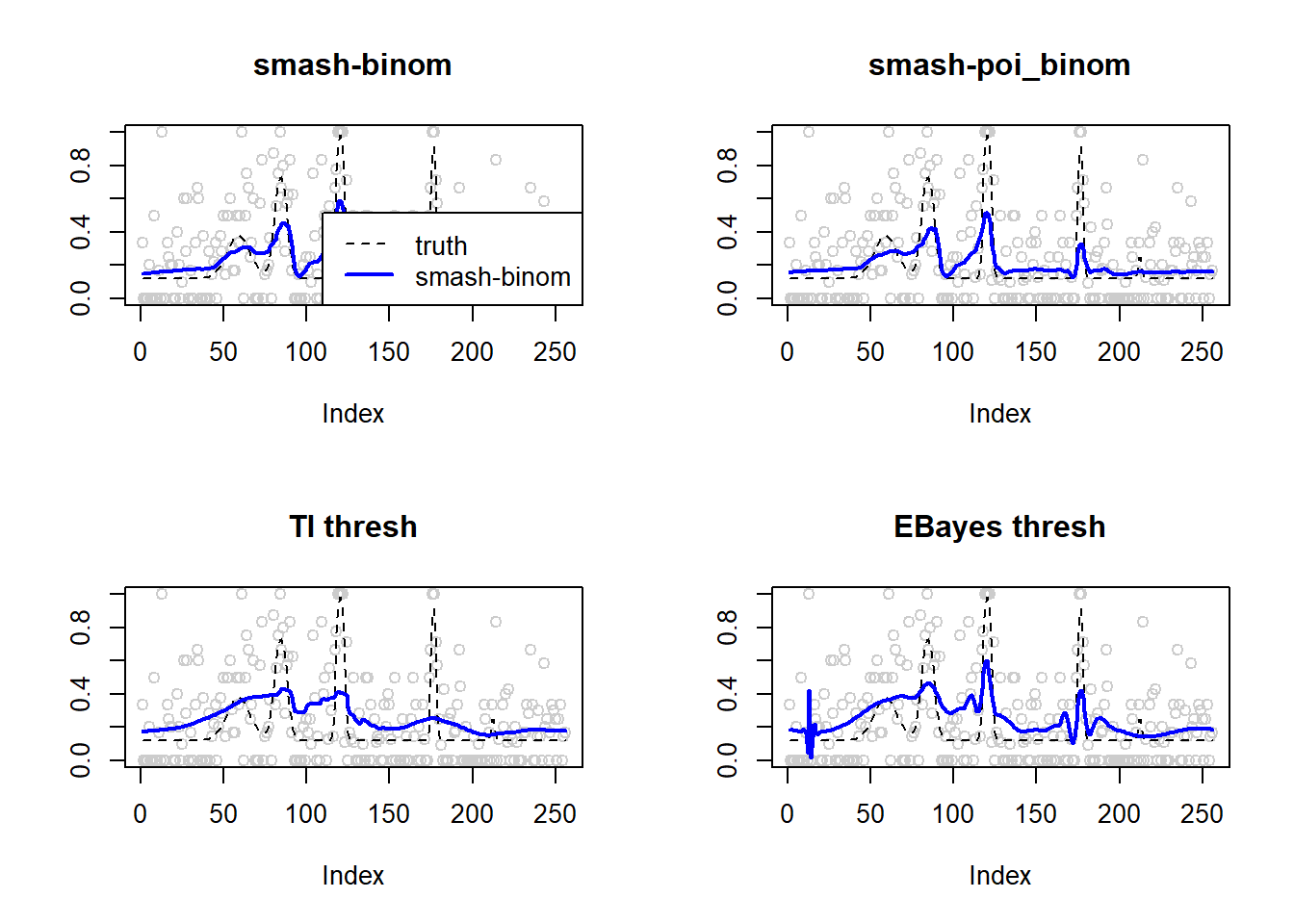
Session information
sessionInfo()R version 3.4.0 (2017-04-21)
Platform: x86_64-w64-mingw32/x64 (64-bit)
Running under: Windows 10 x64 (build 16299)
Matrix products: default
locale:
[1] LC_COLLATE=English_United States.1252
[2] LC_CTYPE=English_United States.1252
[3] LC_MONETARY=English_United States.1252
[4] LC_NUMERIC=C
[5] LC_TIME=English_United States.1252
attached base packages:
[1] stats graphics grDevices utils datasets methods base
other attached packages:
[1] EbayesThresh_1.4-12 ggplot2_2.2.1 smashrgen_0.1.0
[4] wavethresh_4.6.8 MASS_7.3-47 caTools_1.17.1
[7] ashr_2.2-7 smashr_1.1-5
loaded via a namespace (and not attached):
[1] Rcpp_0.12.16 plyr_1.8.4 compiler_3.4.0
[4] git2r_0.21.0 workflowr_1.0.1 R.methodsS3_1.7.1
[7] R.utils_2.6.0 bitops_1.0-6 iterators_1.0.8
[10] tools_3.4.0 digest_0.6.13 tibble_1.3.3
[13] evaluate_0.10 gtable_0.2.0 lattice_0.20-35
[16] rlang_0.1.2 Matrix_1.2-9 foreach_1.4.3
[19] yaml_2.1.19 parallel_3.4.0 stringr_1.3.0
[22] knitr_1.20 REBayes_1.3 rprojroot_1.3-2
[25] grid_3.4.0 data.table_1.10.4-3 rmarkdown_1.8
[28] magrittr_1.5 whisker_0.3-2 backports_1.0.5
[31] scales_0.4.1 codetools_0.2-15 htmltools_0.3.5
[34] assertthat_0.2.0 colorspace_1.3-2 labeling_0.3
[37] stringi_1.1.6 Rmosek_8.0.69 lazyeval_0.2.1
[40] munsell_0.4.3 doParallel_1.0.11 pscl_1.4.9
[43] truncnorm_1.0-7 SQUAREM_2017.10-1 R.oo_1.21.0 This reproducible R Markdown analysis was created with workflowr 1.0.1