Poisson nugget effect, unknown variance
Dongyue Xie
May 13, 2018
Last updated: 2018-05-17
workflowr checks: (Click a bullet for more information)-
✔ R Markdown file: up-to-date
Great! Since the R Markdown file has been committed to the Git repository, you know the exact version of the code that produced these results.
-
✔ Environment: empty
Great job! The global environment was empty. Objects defined in the global environment can affect the analysis in your R Markdown file in unknown ways. For reproduciblity it’s best to always run the code in an empty environment.
-
✔ Seed:
set.seed(20180501)The command
set.seed(20180501)was run prior to running the code in the R Markdown file. Setting a seed ensures that any results that rely on randomness, e.g. subsampling or permutations, are reproducible. -
✔ Session information: recorded
Great job! Recording the operating system, R version, and package versions is critical for reproducibility.
-
Great! You are using Git for version control. Tracking code development and connecting the code version to the results is critical for reproducibility. The version displayed above was the version of the Git repository at the time these results were generated.✔ Repository version: f7f7273
Note that you need to be careful to ensure that all relevant files for the analysis have been committed to Git prior to generating the results (you can usewflow_publishorwflow_git_commit). workflowr only checks the R Markdown file, but you know if there are other scripts or data files that it depends on. Below is the status of the Git repository when the results were generated:
Note that any generated files, e.g. HTML, png, CSS, etc., are not included in this status report because it is ok for generated content to have uncommitted changes.Ignored files: Ignored: .Rhistory Ignored: .Rproj.user/ Ignored: log/ Untracked files: Untracked: analysis/binom.Rmd Untracked: analysis/binomial.Rmd Untracked: analysis/overdis.Rmd Untracked: analysis/smashtutorial.Rmd Untracked: docs/figure/poiunknown.Rmd/ Untracked: docs/figure/sigma.Rmd/ Untracked: docs/figure/smashtutorial.Rmd/ Unstaged changes: Modified: analysis/ashpmean.Rmd Modified: analysis/nugget.Rmd Modified: analysis/unknownvar.Rmd
Expand here to see past versions:
Simulations of Poisson nugget effect(unkown).
Previously, we have studies the methods to estimate unknown \(\sigma\) in the model \(Y_t=\mu_t+N(0,\sigma^2)+N(0,s_t^2)\). Here, we apply mle and smashu methods and compare them with smash as well as smashgen with known \(sigma\). The measure of accuracy is mean square error. Plots are also given as visual aid.
library(smashrgen)
library(ggplot2)
#' Simulation study comparing smash and smashgen
simu_study=function(m,sigma,nsimu=100,seed=12345,
niter=1,family='DaubExPhase',ashp=TRUE,verbose=FALSE,robust=FALSE,
tol=1e-2){
set.seed(seed)
smash.err=c()
smashgen.err=c()
smashgen.smashu.err=c()
smashgen.mle.err=c()
for(k in 1:nsimu){
lamda=exp(m+rnorm(length(m),0,sigma))
x=rpois(length(m),lamda)
#fit data
smash.out=smash.poiss(x)
smashgen.out=smash_gen(x,dist_family = 'poisson',sigma = sigma)
smashu.out=smash_gen(x,dist_family = 'poisson',y_var_est = 'smashu')
mle.out=smash_gen(x,dist_family = 'poisson',y_var_est = 'mle')
smash.err[k]=mse(exp(m),smash.out)
smashgen.err[k]=mse(exp(m),smashgen.out)
smashgen.smashu.err[k]=mse(exp(m),smashu.out)
smashgen.mle.err[k]=mse(exp(m),mle.out)
}
return(list(est=list(smash.out=smash.out,smashgen.out=smashgen.out,smashu.out=smashu.out,mle.out=mle.out,x=x),err=data.frame(smash=smash.err,smashgen=smashgen.err,
smashgen.smashu=smashgen.smashu.err,smashgen.mle=smashgen.mle.err)))
}Simulation 1: Constant trend Poisson nugget
\(\sigma=0.1\)
m=rep(1,128)
result=simu_study(m,0.1)
par(mfrow=c(2,2))
plot(result$est$x,col='gray80',ylab='',main='smash')
lines(exp(m),col=1)
lines(result$est$smash.out,col=4)
plot(result$est$x,col='gray80',ylab='',main='smashgen: known sigma')
lines(exp(m),col=1)
lines(result$est$smashgen.out,col=4)
plot(result$est$x,col='gray80',ylab='',main='smashgen: (sigma^2+s_t^2) from smash')
lines(exp(m),col=1)
lines(result$est$smashu.out,col=4)
plot(result$est$x,col='gray80',ylab='',main='smashgen: sigma from mle')
lines(exp(m),col=1)
lines(result$est$mle.out,col=4)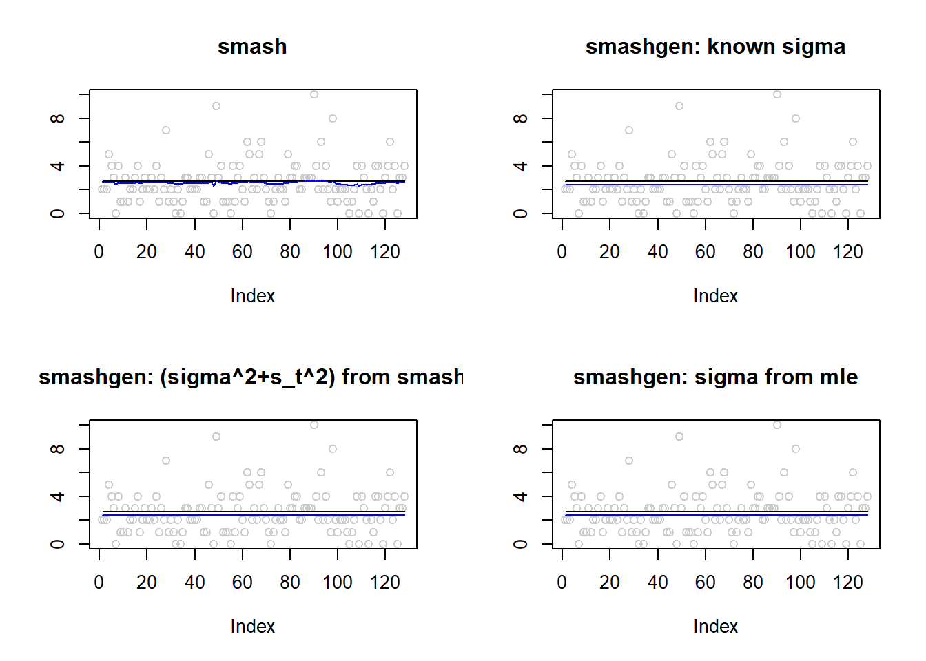
mean(result$err$smash)[1] 0.0318433mean(result$err$smashgen)[1] 0.02987159mean(result$err$smashgen.smashu)[1] 0.03133639mean(result$err$smashgen.mle)[1] 0.02987841ggplot(df2gg(result$err),aes(x=method,y=MSE))+geom_boxplot(aes(fill=method))+labs(x='')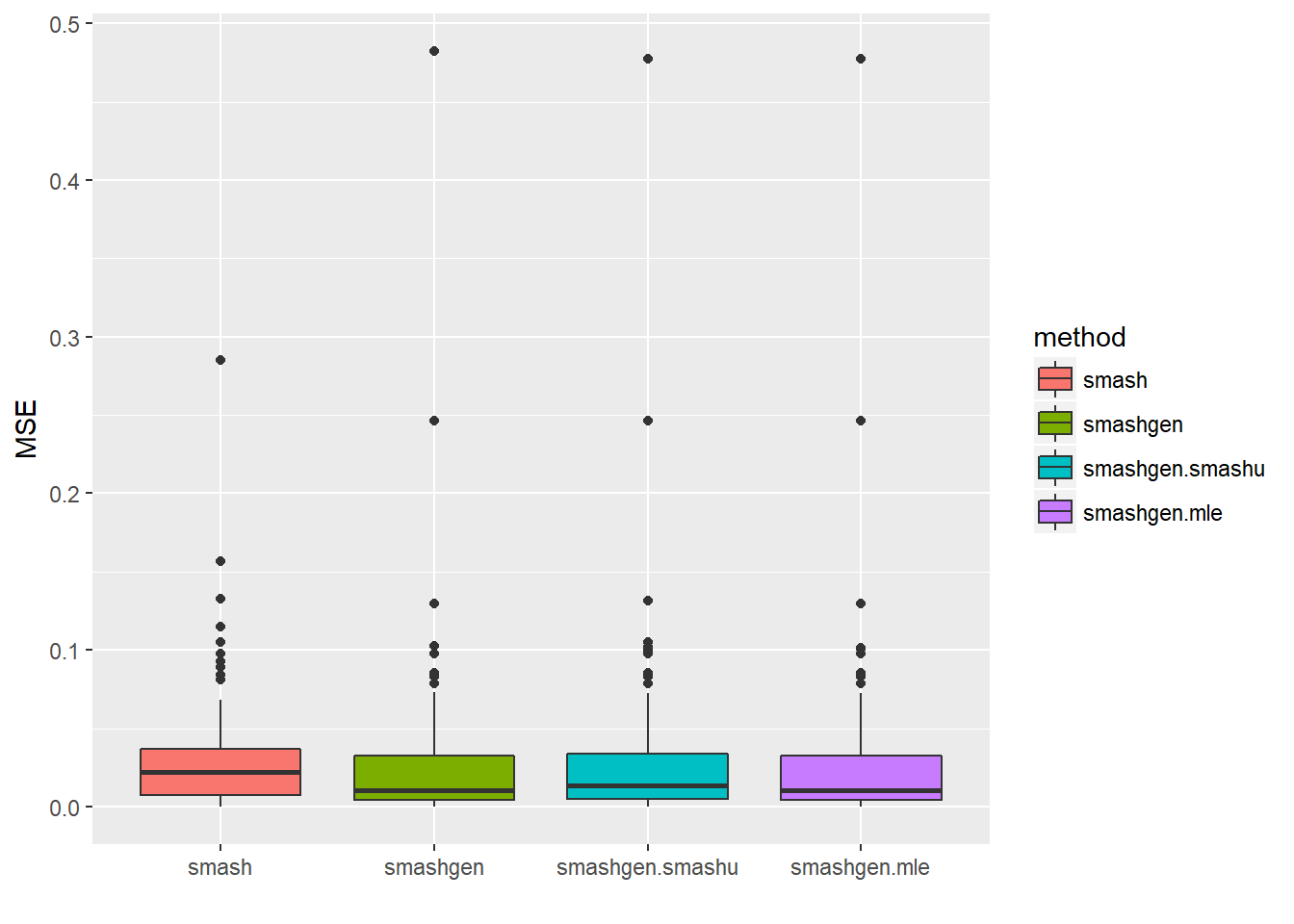
\(\sigma=1\)
m=rep(1,128)
result=simu_study(m,1)
par(mfrow=c(2,2))
plot(result$est$x,col='gray80',ylab='',main='smash')
lines(exp(m),col=1)
lines(result$est$smash.out,col=4)
plot(result$est$x,col='gray80',ylab='',main='smashgen: known sigma')
lines(exp(m),col=1)
lines(result$est$smashgen.out,col=4)
plot(result$est$x,col='gray80',ylab='',main='smashgen: (sigma^2+s_t^2) from smash')
lines(exp(m),col=1)
lines(result$est$smashu.out,col=4)
plot(result$est$x,col='gray80',ylab='',main='smashgen: sigma from mle')
lines(exp(m),col=1)
lines(result$est$mle.out,col=4)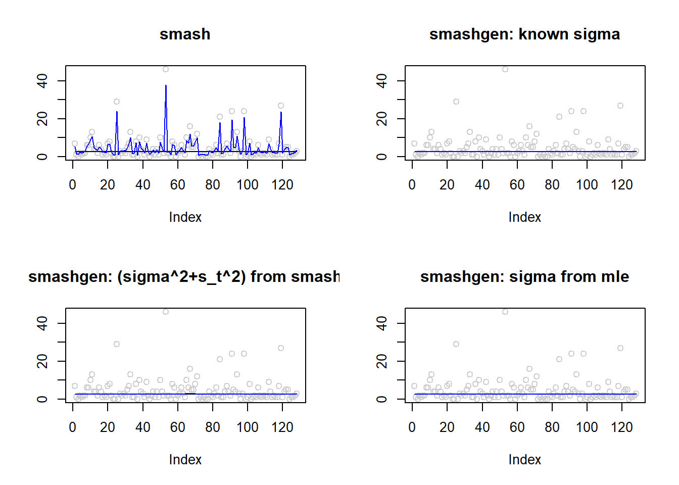
mean(result$err$smash)[1] 29.73513mean(result$err$smashgen)[1] 0.233901mean(result$err$smashgen.smashu)[1] 0.2236465mean(result$err$smashgen.mle)[1] 0.288378#ggplot(df2gg(result$err),aes(x=method,y=MSE))+geom_boxplot(aes(fill=method))+labs(x='')\(\sigma=2\)
m=rep(1,128)
result=simu_study(m,2)
par(mfrow=c(2,2))
plot(result$est$x,col='gray80',ylab='',main='smash')
lines(exp(m),col=1)
lines(result$est$smash.out,col=4)
plot(result$est$x,col='gray80',ylab='',main='smashgen: known sigma')
lines(exp(m),col=1)
lines(result$est$smashgen.out,col=4)
plot(result$est$x,col='gray80',ylab='',main='smashgen: (sigma^2+s_t^2) from smash')
lines(exp(m),col=1)
lines(result$est$smashu.out,col=4)
plot(result$est$x,col='gray80',ylab='',main='smashgen: sigma from mle')
lines(exp(m),col=1)
lines(result$est$mle.out,col=4)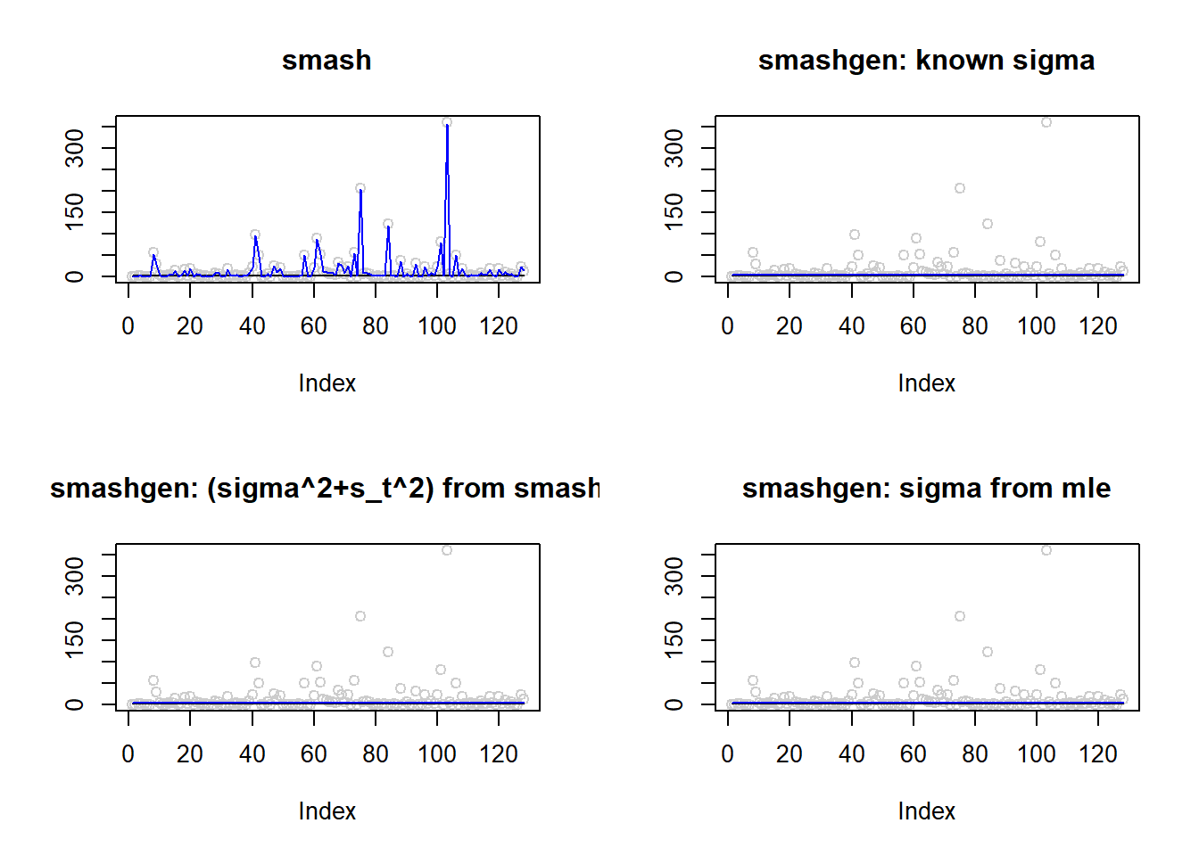
mean(result$err$smash)[1] 8372.27mean(result$err$smashgen)[1] 0.4991542mean(result$err$smashgen.smashu)[1] 0.5850626mean(result$err$smashgen.mle)[1] 0.5626063#ggplot(df2gg(result$err),aes(x=method,y=MSE))+geom_boxplot(aes(fill=method))+labs(x='')Simulation 2: Step trend
\(\sigma=0.1\)
m=c(rep(3,128), rep(5, 128), rep(6, 128), rep(3, 128))
result=simu_study(m,0.1)
par(mfrow=c(2,2))
plot(result$est$x,col='gray80',ylab='',main='smash')
lines(exp(m),col=1)
lines(result$est$smash.out,col=4)
plot(result$est$x,col='gray80',ylab='',main='smashgen: known sigma')
lines(exp(m),col=1)
lines(result$est$smashgen.out,col=4)
plot(result$est$x,col='gray80',ylab='',main='smashgen: (sigma^2+s_t^2) from smash')
lines(exp(m),col=1)
lines(result$est$smashu.out,col=4)
plot(result$est$x,col='gray80',ylab='',main='smashgen: sigma from mle')
lines(exp(m),col=1)
lines(result$est$mle.out,col=4)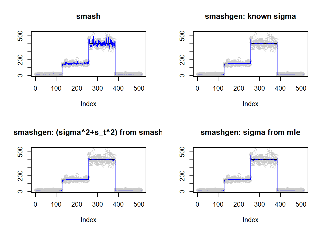
mean(result$err$smash)[1] 368.4722mean(result$err$smashgen)[1] 29.20088mean(result$err$smashgen.smashu)[1] 31.90063mean(result$err$smashgen.mle)[1] 36.42519#ggplot(df2gg(result$err),aes(x=method,y=MSE))+geom_boxplot(aes(fill=method))+labs(x='')\(\sigma=1\)
m=c(rep(3,128), rep(5, 128), rep(6, 128), rep(3, 128))
result=simu_study(m,1)
par(mfrow=c(2,2))
plot(result$est$x,col='gray80',ylab='',main='smash')
lines(exp(m),col=1)
lines(result$est$smash.out,col=4)
plot(result$est$x,col='gray80',ylab='',main='smashgen: known sigma')
lines(exp(m),col=1)
lines(result$est$smashgen.out,col=4)
plot(result$est$x,col='gray80',ylab='',main='smashgen: (sigma^2+s_t^2) from smash')
lines(exp(m),col=1)
lines(result$est$smashu.out,col=4)
plot(result$est$x,col='gray80',ylab='',main='smashgen: sigma from mle')
lines(exp(m),col=1)
lines(result$est$mle.out,col=4)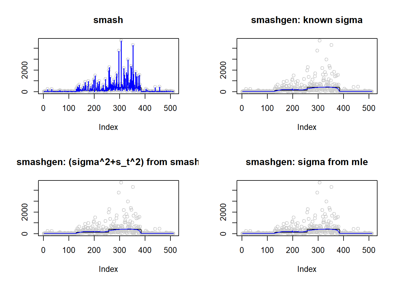
mean(result$err$smash)[1] 223491.6mean(result$err$smashgen)[1] 1658.668mean(result$err$smashgen.smashu)[1] 1650.308mean(result$err$smashgen.mle)[1] 1660.029#ggplot(df2gg(result$err),aes(x=method,y=MSE))+geom_boxplot(aes(fill=method))+labs(x='')Simulation 3: Bumps
\(\sigma=0.1\)
m=seq(0,1,length.out = 256)
h = c(4, 5, 3, 4, 5, 4.2, 2.1, 4.3, 3.1, 5.1, 4.2)
w = c(0.005, 0.005, 0.006, 0.01, 0.01, 0.03, 0.01, 0.01, 0.005,0.008,0.005)
t=c(.1,.13,.15,.23,.25,.4,.44,.65,.76,.78,.81)
f = c()
for(i in 1:length(m)){
  f[i]=sum(h*(1+((m[i]-t)/w)^4)^(-1))
}
m=f
result=simu_study(m,0.1)
par(mfrow=c(2,2))
plot(result$est$x,col='gray80',ylab='',main='smash')
lines(exp(m),col=1)
lines(result$est$smash.out,col=4)
plot(result$est$x,col='gray80',ylab='',main='smashgen: known sigma')
lines(exp(m),col=1)
lines(result$est$smashgen.out,col=4)
plot(result$est$x,col='gray80',ylab='',main='smashgen: (sigma^2+s_t^2) from smash')
lines(exp(m),col=1)
lines(result$est$smashu.out,col=4)
plot(result$est$x,col='gray80',ylab='',main='smashgen: sigma from mle')
lines(exp(m),col=1)
lines(result$est$mle.out,col=4)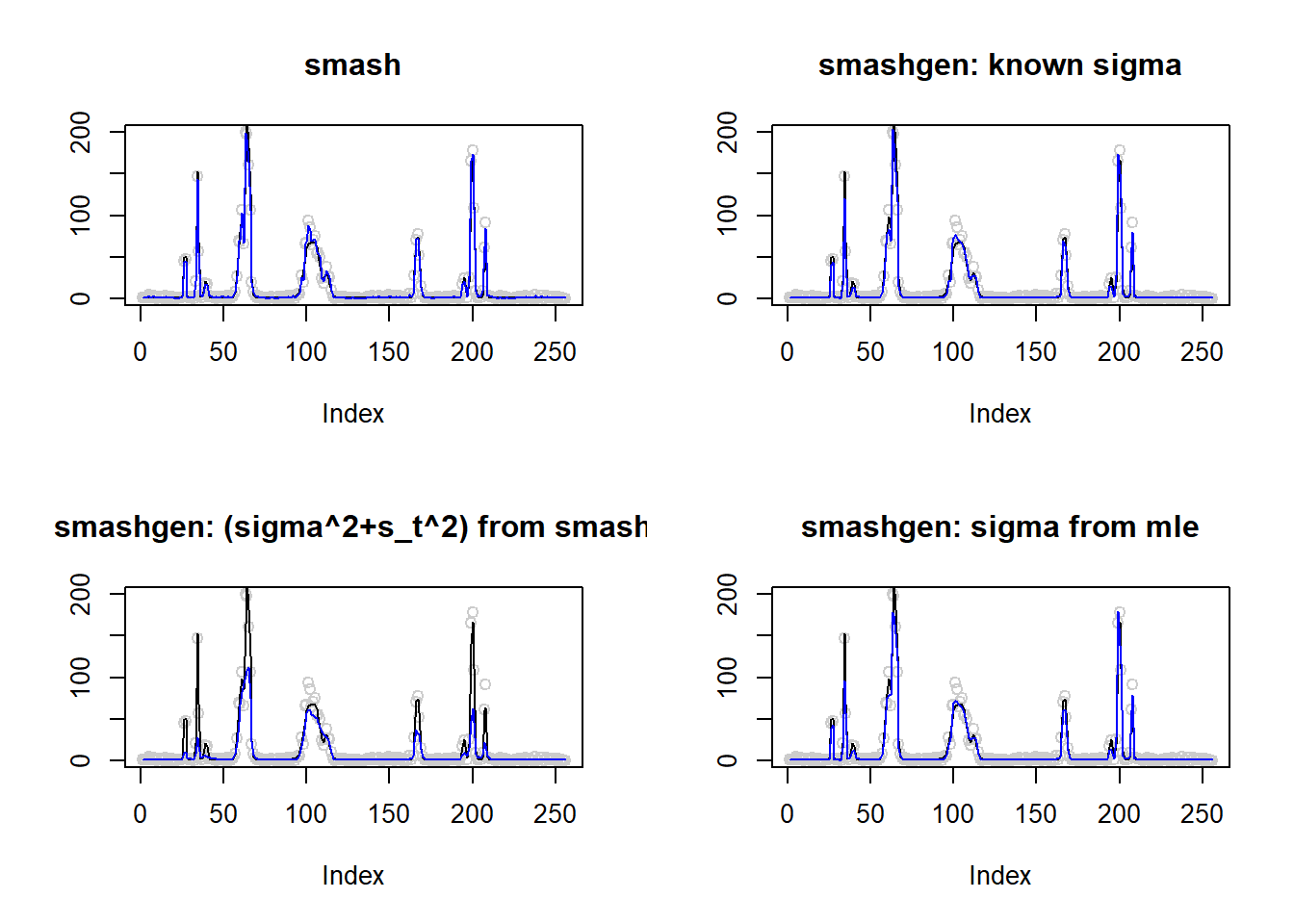
mean(result$err$smash)[1] 23.25972mean(result$err$smashgen)[1] 35.17066mean(result$err$smashgen.smashu)[1] 276.9639mean(result$err$smashgen.mle)[1] 36.6836#ggplot(df2gg(result$err),aes(x=method,y=MSE))+geom_boxplot(aes(fill=method))+labs(x='')\(\sigma=1\)
result=simu_study(m,1)
par(mfrow=c(2,2))
plot(result$est$x,col='gray80',ylab='',main='smash')
lines(exp(m),col=1)
lines(result$est$smash.out,col=4)
plot(result$est$x,col='gray80',ylab='',main='smashgen: known sigma')
lines(exp(m),col=1)
lines(result$est$smashgen.out,col=4)
plot(result$est$x,col='gray80',ylab='',main='smashgen: (sigma^2+s_t^2) from smash')
lines(exp(m),col=1)
lines(result$est$smashu.out,col=4)
plot(result$est$x,col='gray80',ylab='',main='smashgen: sigma from mle')
lines(exp(m),col=1)
lines(result$est$mle.out,col=4)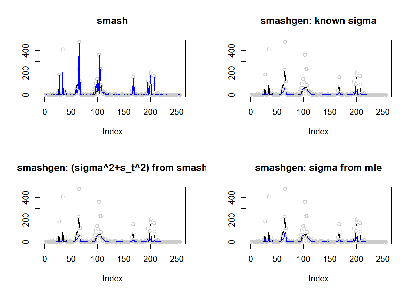
mean(result$err$smash)[1] 6462.494mean(result$err$smashgen)[1] 480.1025mean(result$err$smashgen.smashu)[1] 471.428mean(result$err$smashgen.mle)[1] 856.6609#ggplot(df2gg(result$err),aes(x=method,y=MSE))+geom_boxplot(aes(fill=method))+labs(x='')Simulation 4: Spike mean
\(\sigma=0.1\)
spike.f = function(x) (0.75 * exp(-500 * (x - 0.23)^2) + 1.5 * exp(-2000 * (x - 0.33)^2) + 3 * exp(-8000 * (x - 0.47)^2) + 2.25 * exp(-16000 *
    (x - 0.69)^2) + 0.5 * exp(-32000 * (x - 0.83)^2))
n = 256
t = 1:n/n
m = spike.f(t)

result=simu_study(m,0.1)
par(mfrow=c(2,2))
plot(result$est$x,col='gray80',ylab='',main='smash')
lines(exp(m),col=1)
lines(result$est$smash.out,col=4)
plot(result$est$x,col='gray80',ylab='',main='smashgen: known sigma')
lines(exp(m),col=1)
lines(result$est$smashgen.out,col=4)
plot(result$est$x,col='gray80',ylab='',main='smashgen: (sigma^2+s_t^2) from smash')
lines(exp(m),col=1)
lines(result$est$smashu.out,col=4)
plot(result$est$x,col='gray80',ylab='',main='smashgen: sigma from mle')
lines(exp(m),col=1)
lines(result$est$mle.out,col=4)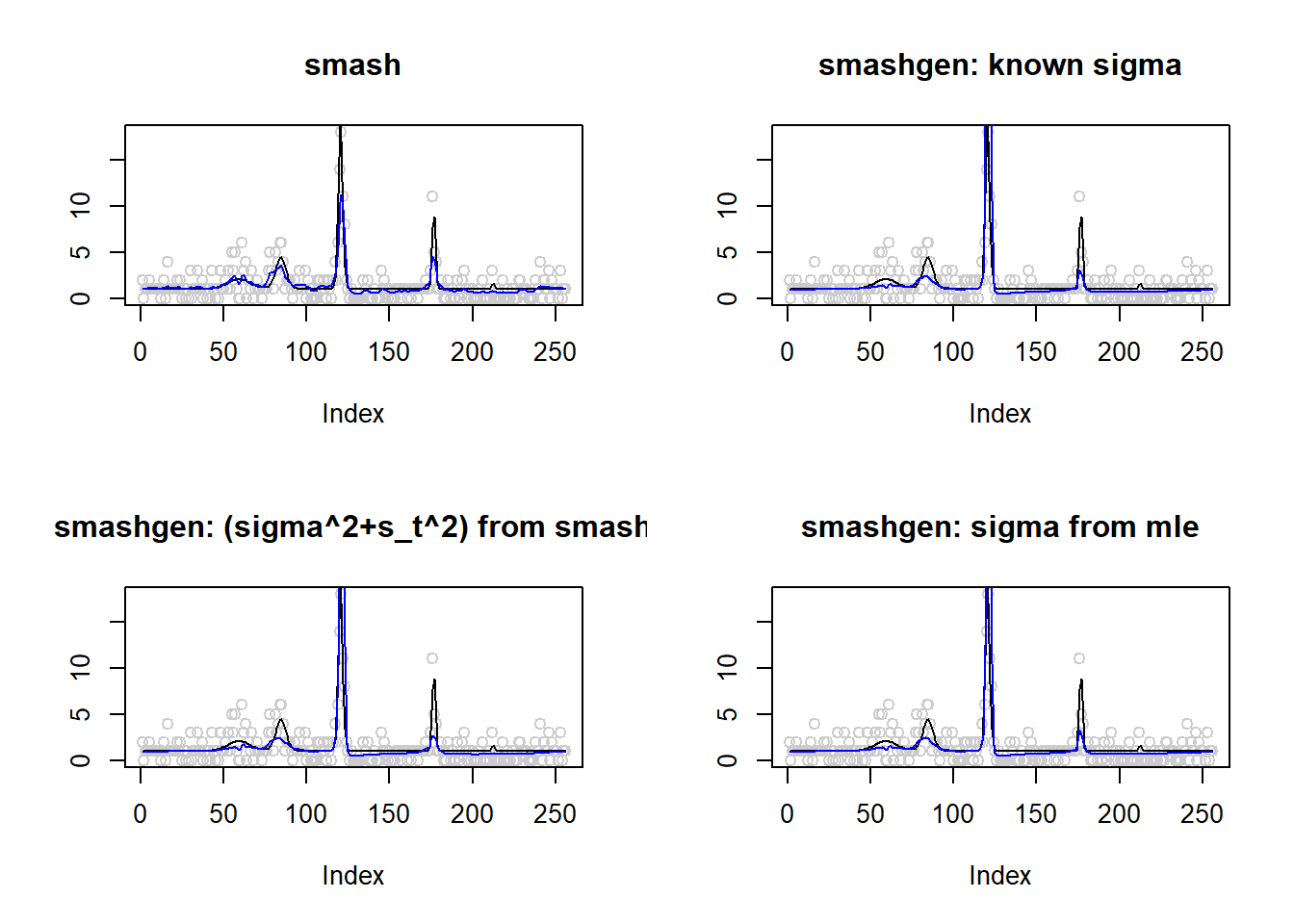
mean(result$err$smash)[1] 0.6011156mean(result$err$smashgen)[1] 12306.79mean(result$err$smashgen.smashu)[1] 2931.977mean(result$err$smashgen.mle)[1] 12630.5#ggplot(df2gg(result$err),aes(x=method,y=MSE))+geom_boxplot(aes(fill=method))+labs(x='')\(\sigma=1\)
result=simu_study(m,1)
par(mfrow=c(2,2))
plot(result$est$x,col='gray80',ylab='',main='smash')
lines(exp(m),col=1)
lines(result$est$smash.out,col=4)
plot(result$est$x,col='gray80',ylab='',main='smashgen: known sigma')
lines(exp(m),col=1)
lines(result$est$smashgen.out,col=4)
plot(result$est$x,col='gray80',ylab='',main='smashgen: (sigma^2+s_t^2) from smash')
lines(exp(m),col=1)
lines(result$est$smashu.out,col=4)
plot(result$est$x,col='gray80',ylab='',main='smashgen: sigma from mle')
lines(exp(m),col=1)
lines(result$est$mle.out,col=4)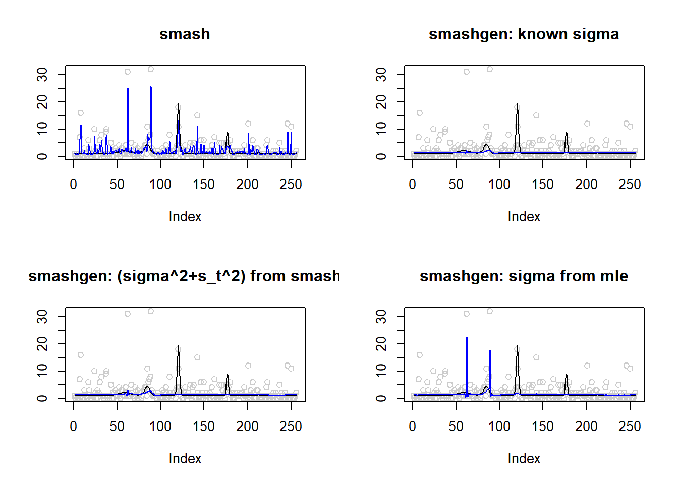
mean(result$err$smash)[1] 34.61266mean(result$err$smashgen)[1] 7991947410mean(result$err$smashgen.smashu)[1] 4418267884mean(result$err$smashgen.mle)[1] 13168337929#ggplot(df2gg(result$err),aes(x=method,y=MSE))+geom_boxplot(aes(fill=method))+labs(x='')Session information
sessionInfo()R version 3.4.0 (2017-04-21)
Platform: x86_64-w64-mingw32/x64 (64-bit)
Running under: Windows 10 x64 (build 16299)
Matrix products: default
locale:
[1] LC_COLLATE=English_United States.1252
[2] LC_CTYPE=English_United States.1252
[3] LC_MONETARY=English_United States.1252
[4] LC_NUMERIC=C
[5] LC_TIME=English_United States.1252
attached base packages:
[1] stats graphics grDevices utils datasets methods base
other attached packages:
[1] ggplot2_2.2.1 smashrgen_0.1.0 wavethresh_4.6.8 MASS_7.3-47
[5] caTools_1.17.1 ashr_2.2-7 smashr_1.1-5
loaded via a namespace (and not attached):
[1] Rcpp_0.12.16 plyr_1.8.4 compiler_3.4.0
[4] git2r_0.21.0 workflowr_1.0.1 R.methodsS3_1.7.1
[7] R.utils_2.6.0 bitops_1.0-6 iterators_1.0.8
[10] tools_3.4.0 digest_0.6.13 tibble_1.3.3
[13] evaluate_0.10 gtable_0.2.0 lattice_0.20-35
[16] rlang_0.1.2 Matrix_1.2-9 foreach_1.4.3
[19] yaml_2.1.19 parallel_3.4.0 stringr_1.3.0
[22] knitr_1.20 REBayes_1.3 rprojroot_1.3-2
[25] grid_3.4.0 data.table_1.10.4-3 rmarkdown_1.8
[28] magrittr_1.5 whisker_0.3-2 backports_1.0.5
[31] scales_0.4.1 codetools_0.2-15 htmltools_0.3.5
[34] assertthat_0.2.0 colorspace_1.3-2 labeling_0.3
[37] stringi_1.1.6 Rmosek_8.0.69 lazyeval_0.2.1
[40] munsell_0.4.3 doParallel_1.0.11 pscl_1.4.9
[43] truncnorm_1.0-7 SQUAREM_2017.10-1 R.oo_1.21.0 This reproducible R Markdown analysis was created with workflowr 1.0.1