Logistic Regression With Regularization

Ann Arbor R User Group, April 2015

Devin Riley

Overview

  • Brief intro to logistic regression
  • Motivation for regularization techniques
  • Explanation of the most common regularization techniques:
    • Ridge regression
    • Lasso regression
  • An example of each on a sample dataset


R packages to install if you want to follow along:

pkgs <- c('glmnet', 'ISLR')
install.packages(pkgs)
Logistic Regression

Widely utilized classification technique.
Regression for when the response variable is qualitative.
Special case of the general linear model.
For a response \(y\), model the probability that \(y\) belongs to a particular class or category.

\[y \in \{0, 1\}\]

With respect to a simple linear regression, we can think of it as: \[p^'_\beta(x) = \beta^T x = \beta_0 + \beta_1 x_1 + ... + \beta_p x_p\]

Where we would like \(p^'_\beta(x)\) to represent the probability that x belongs to a particular class
But, this formulation does not fit the definition of probability (i.e. on [0,1]), so need model representation, \(p_\beta(x)\) s.t.:

\[ 0 \le p_\beta \le 1\]

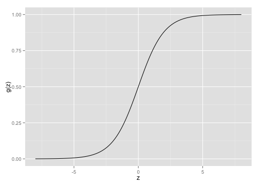
The logistic function

AKA Sigmoid function:
\[g(z) = \dfrac{1}{1 + e^{-z}}\]

plot of chunk unnamed-chunk-2

Logistic Regression

So if our original representation was
\[p^'_\beta(x) = \beta^T x\] then our representation becomes
\[p_\beta(x) = g(p^'_\beta(x)) = g(\beta^T x)\]

where g(z), again, is \[g(z) = \dfrac{1}{1 + e^{-z}}\]

Logistic Regression

So, \[p_\beta(x) = \dfrac{1}{1 + e^{-\beta^T x}}\]

After a bit of manipulation, we have
\[ \dfrac{p_\beta(x)}{1-p_\beta(x)} = e^{\beta^T x}\] which is the "odds" function. And taking the logarithm of both sides, we have \[\log\Big(\dfrac{p_\beta(x)}{1-p_\beta(x)}\Big) = \beta^T x\] which is the "log-odds" or logit and gives us the desired property.

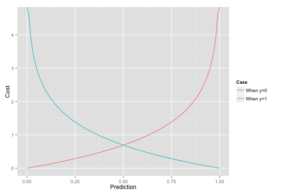
The cost function

\[Cost(p_\beta(x), y) = \begin{cases} -log(p_\beta(x)) & \text{if }y=1 \\ -log(1 - p_\beta(x)) & \text{if }y=0 \end{cases} \]

plot of chunk unnamed-chunk-3

The cost function


We can rewrite the cost function in a simpler form as

\[Cost(p_\beta(x), y) = -ylog(p_\beta(x)) - (1-y)log(1-p_\beta(x))\]

Since when

  • y=1 then \(Cost(p_\beta(x), y) = -log(p_\beta(x))\)
  • y=0 then \(Cost(p_\beta(x), y) = -log(1 - p_\beta(x))\)

Motivation For Regularization

If our \(\beta_j\)'s are unconstrained:

  • They can explode, become very big
  • Are subject to high variance

To control this variance, we can regularize these coefficients.
And so we can think about this regularization in terms of the bias-variance tradeoff.

If our \(\beta_j\)'s are subject to high variance, then we are overfitting our model to the particular quirks or noise in our dataset. So we wish to trade bias, in the form of regularization, to control this variance.

Not obvious that shrinking parameters does this for us.
And, of course, we don't know which ones to shrink a priori!

Ridge regression

  • Recall our original logistic regression cost function to be:
    \[Cost(p_\beta(x), y) = -ylog(p_\beta(x)) - (1-y)log(1-p_\beta(x))\]

  • Ridge regression adds a penalty to this cost that is a function of the coefficient sizes:
    \[Cost_R(p_\beta(x), y) = -ylog(p_\beta(x)) - (1-y)log(1-p_\beta(x)) + \color{blue}{\lambda\sum_{j=1}^{p} \beta_j^2}\]

  • \(\lambda\) is the shrinkage parameter

    • Controls the regularization
    • \(\lambda\rightarrow0\) gives us regular logistic regression, \(\lambda\rightarrow\infty\) null model
  • \(||\beta||_2 = \sum_{j=1}^{p} \beta_j^2\) is called L2 Norm.

Hitters dataset from ISLR package

Hitters <- ISLR::Hitters
dim(Hitters)
## [1] 322  20
Hitters[1, ]
##                AtBat Hits HmRun Runs RBI Walks Years CAtBat CHits CHmRun
## -Andy Allanson   293   66     1   30  29    14     1    293    66      1
##                CRuns CRBI CWalks League Division PutOuts Assists Errors
## -Andy Allanson    30   29     14      A        E     446      33     20
##                Salary NewLeague
## -Andy Allanson     NA         A

Prep data for model building

library(ISLR)

# Remove NA
Hitters <- na.omit(ISLR::Hitters)
dim(Hitters)
## [1] 263  20
set.seed(42)
train<-sample(1:nrow(Hitters), .6*nrow(Hitters))
test<-(-train)

# Convert Salary to a binary factor variable
Hitters$Salary <- factor(as.numeric(Hitters$Salary > 500))

Ridge regression example

library(ISLR)
library(glmnet)

x <- model.matrix(Salary~., Hitters)[,-1]
y <- Hitters$Salary

grid=10^seq(-6,2,length=100)
ridge.mod <- glmnet(x[train,], y[train], family="binomial", alpha=0, lambda=grid)
# family="binomial" => classification, same as glm
# alpha=0 gives us the ridge regularization
# lambda is the regularization parameter

Ridge regression example

class(ridge.mod)
## [1] "lognet" "glmnet"
dim(coef(ridge.mod))
## [1]  20 100

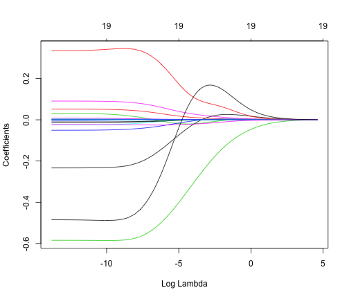
Ridge regression example

plot(ridge.mod, xvar="lambda")

plot of chunk unnamed-chunk-9

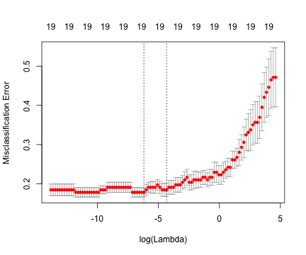
Choosing regularization parameter \(\lambda\)

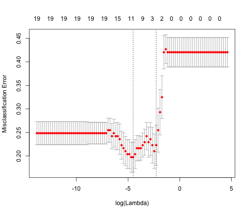
Use cross-validation to determine the appropriate \(\lambda\)

cv.ridgemod <- cv.glmnet(x[train, ], y[train], family="binomial", 
                         alpha=0, type.measure="class", lambda=grid)
plot(cv.ridgemod)

plot of chunk unnamed-chunk-10

Improvement over basic logistic regression?

best_lambda <- cv.ridgemod$lambda.min
ridge.pred <- predict(ridge.mod, s=best_lambda, newx=x[test, ], type="response")
table(round(ridge.pred), y[test])
##    
##      0  1
##   0 51 19
##   1  9 27

for an accuracy of 0.7358. Running a plain-old logistic regression using glm() gives us an accuracy of 0.7264, and so the ridge regularization provides a moderate improvement in accuracy.

Lasso regression

Least Absolute Shrinkage and Selection Operator
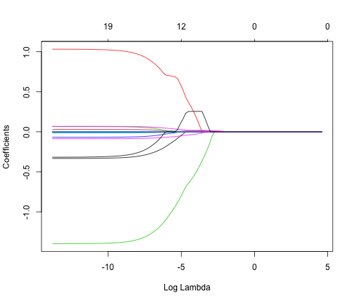
Coefficients can be set exactly to 0, and so it performs variable selection
This can help with interpretability, especially when # of predictors is large

\[Cost_L(p_\beta(x), y) = -ylog(p_\beta(x)) - (1-y)log(1-p_\beta(x)) + \color{blue}{\lambda\sum_{j=1}^{p} \left|\beta_j\right|}\]

\(||\beta||_1 = \sum_{j=1}^{p} \left|\beta_j\right|\) is the L1 Norm
Similar to ridge:

  • \(\lambda\rightarrow0\) gives us regular logistic regression
  • \(\lambda\rightarrow\infty\) gives us null model
  • But, behavior inbetween is quite different

Lasso regression example

lasso.mod <- glmnet(x[train, ], y[train], lambda=grid, 
                family="binomial", alpha=1)
plot(lasso.mod, xvar="lambda")

plot of chunk unnamed-chunk-13

Lasso regression example

cv.lassomod <- cv.glmnet(x[train, ], y[train], lambda=grid,
                       family="binomial", alpha=1, type.measure="class")
plot(cv.lassomod)

plot of chunk unnamed-chunk-14

Lasso performance

lbest_lambda <- cv.lassomod$lambda.min
new.prob <- predict(lasso.mod, newx=x[test, ], s=lbest_lambda, type="response")
new.class <- round(new.prob)
table(factor(new.class), y[test])
##    
##      0  1
##   0 54 18
##   1  6 28

Which gives us an accuracy of 0.7736, which out-performs both the performance of the original logistic regression and the ridge regression (with accuracies of 0.7264 and 0.7358, respectively).

Model selection!

## 19 x 1 sparse Matrix of class "dgCMatrix"
##                    s0
## AtBat       0.0022191
## Hits        0.0102524
## HmRun       .        
## Runs        .        
## RBI         .        
## Walks       0.0195095
## Years       .        
## CAtBat      .        
## CHits       0.0018991
## CHmRun      .        
## CRuns       .        
## CRBI        .        
## CWalks      .        
## LeagueN     0.3675261
## DivisionW  -0.6408992
## PutOuts     0.0007079
## Assists    -0.0003869
## Errors     -0.0396275
## NewLeagueN  0.2537524

Resources